Machine learning often ends up with a mathematical optimization problem, typically minimizing a cost function $J(\mathbf{w})$ for a given parameter $\mathbf{w} = \begin{bmatrix} w_0 & w_1 & \cdots & w_n \end{bmatrix}^{T} \in \mathbb{R}^{n+1}$ that has the form:
$$ J(\mathbf{w})=\frac{1}{M} \sum_{m=1}^{M} J_m(\mathbf{w}). \tag{opt:1}\label{eq:opt} $$
Here, $J_m(\mathbf{w})$ is the cost associated with the $m$-th observation in a training set, and $M$ denotes the total number of observations. Thus, one can say that given the parameter $\mathbf{w}$, the cost function $J(\mathbf{w})$ represents the average cost over all observations in the training set. Among all the possible parameters, the one that results in the smallest value of the cost function is called the minimizer, or solution, and we denote it by $\mathbf{w}^{*}$. The term “learning” in the machine learning means a procedure for finding the solution $\mathbf{w}^{*}$.
Gradient descent
Now, how can we find the solution $\mathbf{w}^{*}$ to \eqref{eq:opt}? One simple way is the gradient descent. The method of gradient descent is to find a local minimum of a cost function $J(\mathbf{w})$, taking steps in the opposite direction to the gradient $\nabla{J(\mathbf{w})}$, where
$$
\nabla{J(\mathbf{w})})=
\begin{bmatrix}
\frac{\partial}{\partial w_0} J(\mathbf{w}) \\
\frac{\partial}{\partial w_1} J(\mathbf{w}) \\
\vdots \\
\frac{\partial}{\partial w_n} J(\mathbf{w})
\end{bmatrix}.
$$
Consider the Taylor series of $J(\mathbf{w}-\alpha \nabla{J(\mathbf{w})})$ as a function of $\alpha$: $$J(\mathbf{w}-\alpha \nabla{J(\mathbf{w})})=J(\mathbf{w})-\alpha\Vert \nabla{J(\mathbf{w})}\Vert^2 + o(\alpha).$$ If $\nabla{J(\mathbf{w})} \ne 0$, then for sufficiently small $\alpha>0$, we have $$J(\mathbf{w}-\alpha \nabla{J(\mathbf{w})})<J(\mathbf{w}).$$ This means that the parameter $\mathbf{w}-\alpha \nabla{J(\mathbf{w})}$ leads to the smaller value of the cost function than the parameter $\mathbf{w}$. Intuitively, the gradient $\nabla{J(\mathbf{w})}$ is the direction of the maximum rate of increase at the parameter $\mathbf{w}$, so moving in the opposite direction lowers the value of the cost function.
Thus, we can start with a random guess $\mathbf{w}^{(0)}$ and keep moving to $\mathbf{w}^{(1)}$, $\mathbf{w}^{(2)}$, $\ldots$, $\mathbf{w}^{(t)}$ in such a way that $$ \mathbf{w}^{(t+1)} = \mathbf{w}^{(t)}-\alpha \nabla{J(\mathbf{w}^{(t)})}, \tag{opt:2}\label{eq:gd} $$ or in other form $$ w_{j}^{(t+1)} = w_{j}^{(t)}-\alpha \left. \frac{\partial J(\mathbf{w})}{\partial w_{j}} \right\vert_{\mathbf{w}=\mathbf{w}^{(t)}}\text{ for all } j. \label{eq:gd_element} $$ Then, for sufficiently small $\alpha>0$, we have, for every $t$, $$J(\mathbf{w}^{(t+1)}) < J(\mathbf{w}^{(t)}),$$ and $\mathbf{w}^{(t)}$ converges to a local minimum as $t$ grows. When the cost function $J(\mathbf{w})$ is convex, the local minimum is also the global minimum, so in such a case, $\mathbf{w}^{(t)}$ can converge to the solution $\mathbf{w}^{*}$. For non-convex cost functions, the gradient descent does not guarantee us finding the global minimum. Instead, depending on the initial guess, we will end up with different local minimum, which is exemplified in Figure 1.
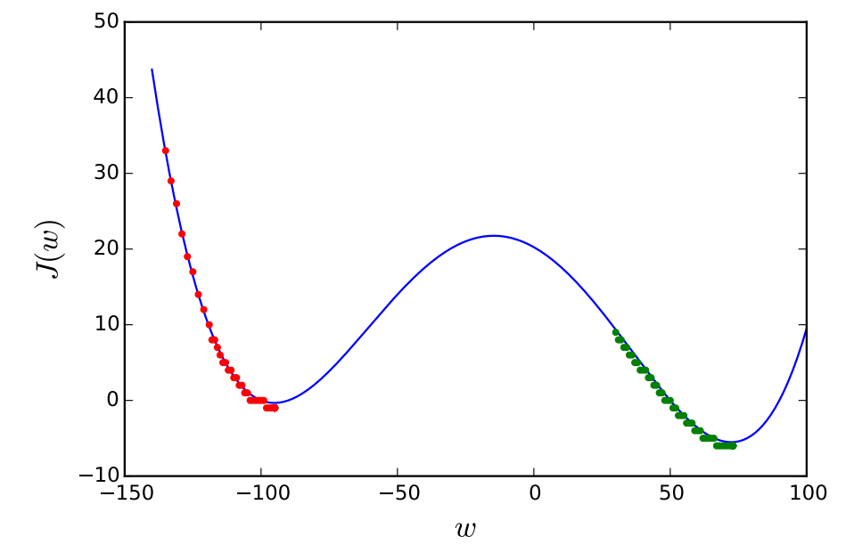
The effect of the initial guess when $J(w)=(w+90)(w-50)(w/2+50)(w-90)/1000000$.
The red and green dots represent the trajectories of the gradient descent corresponding to the initial values $w^{(0)}=-135$ and $w^{(0)}=30$, respectively.
Learning rate
In \eqref{eq:gd}, the value of $\alpha$ is called the learning rate. This value determines how fast or slow the parameter moves towards the optimal solution. Figure 2 illustrates the effect of the learning rate.
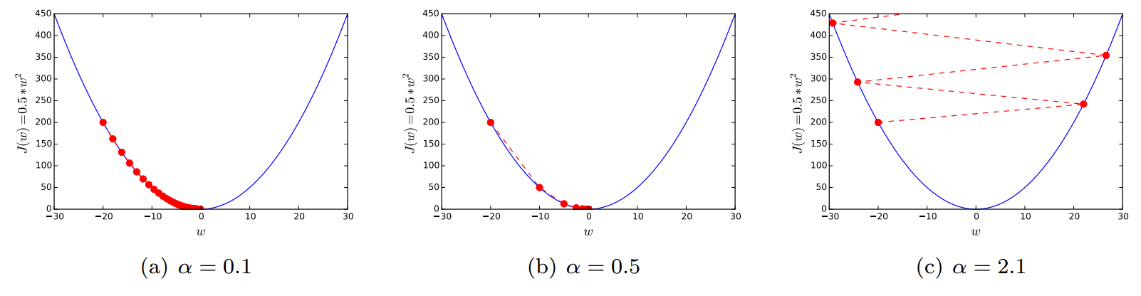
The effect of the learning rate when $J(w)=\frac{1}{2}w^2$ and $w^{(0)}=-20$.
If $\alpha$ is too small, the gradient descent may take too long to converge. In contrast, the gradient descent may fail to converge with too large value of $\alpha$.
Choosing the proper value of the learning rate is not that trivial. In practice, we often use simply a small enough constant by keeping decreasing the value until the parameter seems to converge to a certain point. Or in order to get more accurate solution, one can halve the value of the learning rate as convergence slows down over iterations. Another method is to adaptively change the learning rate at every iteration $t$ in the way that the difference $ J(\mathbf{w}^{(t)})-J(\mathbf{w}^{(t+1)})$ is maximized. For more detail on this method, refer to the steepest descent.
Stochastic gradient descent
From \eqref{eq:opt}, the gradient $\nabla{J(\mathbf{w})}$ is represented as $$ \nabla{J(\mathbf{w})}=\frac{1}{M} \sum_{m=1}^{M} \nabla{J_m(\mathbf{w})}. \label{eq:gradient} $$ This implies that computing $\nabla{J(\mathbf{w})}$ is equivalent to taking the average of $\nabla{J_m(\mathbf{w})}$, the gradient of the cost specific to the $m$-th observation, over the full training set. However, in practice, the training set is often very large, and thus averaging over the entire set can take a significant time. For this reason, the stochastic gradient descent simply approximates the true gradient by a gradient at a single observation as follows: $$\nabla{J(\mathbf{w})}\approxeq\nabla{J_m(\mathbf{w})}. \label{eq:gradient_approx}$$ Thus, with the stochastic gradient descent, the parameter update equation in \eqref{eq:gd} can be rewritten as $$ \mathbf{w}^{(t+1)} = \mathbf{w}^{(t)}-\alpha \nabla{J_t(\mathbf{w}^{(t)})}. \label{eq:sto_gd} $$
As a compromise between the true gradient and the gradient at a single observation, one may also consider the gradient averaged over a few training samples.
Practice
Tensorflow provides a function that implements the gradient descent algorithm. Thus, you can just use it without deriving an actual gradient. What you need to do is to choose the value of the learning rate. The following shows an example.
import tensorflow as tf
import numpy as np

w = tf.Variable(100.0)  # initial guess = 100.0
J = tf.pow(w, 2)        # J(w) = w^2

optimizer = tf.train.GradientDescentOptimizer(0.05)     # learning rate = 0.05
train = optimizer.minimize(J)

# Initialize variables
init = tf.initialize_all_variables()

sess = tf.InteractiveSession()
sess.run(init)

for step in range(0, 201):
    sess.run(train)
    if step % 20 == 0:
        print "%3d, %10.5f, %10.5f" % (step, w.eval(), J.eval())

sess.close()
The output of the script would be as follows:
  0,   90.00000, 8100.00000
 20,   10.94190,  119.72514
 40,    1.33028,    1.76964
 60,    0.16173,    0.02616
 80,    0.01966,    0.00039
100,    0.00239,    0.00001
120,    0.00029,    0.00000
140,    0.00004,    0.00000
160,    0.00000,    0.00000
180,    0.00000,    0.00000
200,    0.00000,    0.00000