Linear regression is a means of modeling the relationship between one or more independent variables (inputs) and a single dependent variable (an output) by fitting a linear equation to observed data.
Hypothesis function
Given the $m$-th observation with inputs $\{ x_{m,1}, x_{m,2}, \ldots, x_{m,n} \}$ where $x_{m,j} \in \mathbb{R}, \forall j$ and an output $y_m \in \mathbb{R}$, we define an input vector as
$$
\mathbf{x}_m=
\begin{bmatrix}
x_{m,0} \\
x_{m,1} \\
\vdots \\
x_{m,n}
\end{bmatrix} \in \mathbb{R}^{n+1},
\label{eq:input_vector}
$$
where we always set $x_{m,0}=1$, which is called a bias input and considered here for notational convenience. The goal of linear regression is to find an estimate $\hat{y}_m=h_{\mathbf{w}}(\mathbf{x}_{m})$ of the output $y_{m}$ that is of the form:
$$ h_{\mathbf{w}}(\mathbf{x}_{m})=\mathbf{w}^T \mathbf{x}_{m}=w_0 + w_1 x_{m,1} + \ldots +w_n x_{m,n}. $$
We call $h_{\mathbf{w}}(\cdot)$ a hypothesis function. By well choosing the value of $\mathbf{w}$, we want $h_{\mathbf{w}}(\mathbf{x}_{m})$ as close to $y_{m}$ as possible for $m=1,2,\ldots,M$. Again, $M$ is the number of observations in the training set.
Note that when $n=1$, the hypothesis function is represented as
$$ h_{\mathbf{w}}(\mathbf{x}_{m})=w_0 + w_1 x_{m,1}, $$
which is the form of a straight line. Thus, all we need to do here is to find the slope $w_1$ and the $y$-intercept $w_0$ of a straight line that fits best to given points ${(x_{m,1}, y_{m})}_{m=1}^{M}$. This case is called simple linear regression. Figure 1 shows an example of the simple linear regression.
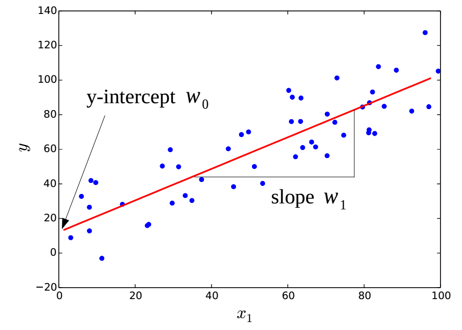
Simple linear regression.
The blue dots represent the training data ${(x{m,1}, y{m})}_{m=1}^{M}$. The result of the simple linear regression is the red line
Cost function
We need a measure of how “well” we have selected the value of $\mathbf{w}$. To this end, the cost function $J(\mathbf{w})$ can be defined as
$$ J(\mathbf{w})=\frac{1}{M} \sum_{m=1}^{M} \left(h_{\mathbf{w}}(\mathbf{x}_{m})-y_{m} \right)^{2}. \tag{lr:1}\label{eq:mse} $$
Saying the value of $h_{\mathbf{w}}(\mathbf{x}_{m})-y_{m}$ is an error, the cost function above is the mean of squared errors. Then, the best value of $\mathbf{w}$, i.e., the solution $\mathbf{w}^{*}$, is chosen as the one that minimizes the cost function $J(\mathbf{w})$ in \eqref{eq:mse}. Such a solution is said to be optimal in the sense of minimizing mean-squared errors (MMSE).
Learning
Formally, the solution $\mathbf{w}^{*}$ is obtained as $$ \mathbf{w}^{*}=\arg \min_{\mathbf{w}} J(\mathbf{w}). $$
This can be solved numerically by using the gradient descent. Since $$ J(\mathbf{w})=\frac{1}{M} \sum_{m=1}^{M} \left(w_0 + w_1 x_{m,1} + \ldots +w_n x_{m,n}-y_{m} \right)^{2}, $$
we have $$ \frac{\partial}{\partial w_j} J(\mathbf{w})= \frac{2}{M} \sum_{m=1}^{M} \left(w_0 + w_1 x_{m,1} + \ldots +w_n x_{m,n}-y_{m} \right)x_{m,j}. $$ Therefore, from (opt:1), the gradient descent equations for linear regression are
$$ w_{j}^{(t+1)}=w_{j}^{(t)}-\alpha\frac{2}{M} \sum_{m=1}^{M} \left(w_0^{(t)} + w_1^{(t)} x_{m,1} + \ldots +w_n^{(t)} x_{m,n}-y_{m} \right)x_{m,j} $$
for all $j$.
Prediction
After we have found the solution $\mathbf{w}^{*}$, if an additional input vector $\mathbf{x} = \begin{bmatrix} 1 & x_1 & \ldots & x_n \end{bmatrix}^{T}$ is given, its corresponding output $y$ can be predicted as follows:
$$ y=h_{\mathbf{w}^{*}}(\mathbf{x})=w_0^{*} + w_1^{*} x_1 + \ldots +w_n^{*} x_n = \mathbf{w}^{*T} \mathbf{x}. $$
Practice
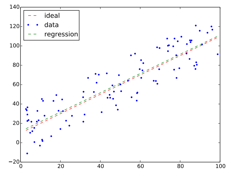
The following code show an example of the simple lienar gression. Data used for training is created by adding noises around the straight line of y-intercept=10 and slope=1. The output would be like Figure 2.
import numpy as np
import matplotlib.pyplot as plt
import tensorflow as tf

n_data = 100
r_x = 100
noise_std = 50
x = None
y = None
y_ideal = None
#----------------------------------------------------------------
def create_data():
    global x, y, y_ideal
    y_intercept = 10
    slope = 1
    x = np.float32(np.random.rand(n_data)) * r_x
    x = np.sort(x)
    noise = (np.float32(np.random.rand(n_data)) - 0.5) * noise_std
    y_ideal = slope * x + y_intercept
    y = y_ideal + noise
#----------------------------------------------------------------
def draw(w1, w0):
    y_hat = w1 * x + w0

    plt.plot(x[:], y_ideal[:], 'r--', \
             x[:], y[:], 'b.',\
             x[:], y_hat[:], 'g--')

    plt.xlim(0, r_x)
    plt.legend(['ideal', 'data', 'regression'], loc='best')
    plt.savefig('linear_one.pdf')
#----------------------------------------------------------------

# Create data for training
create_data()

# Model
w_1 = tf.Variable(np.random.rand())
w_0 = tf.Variable(np.random.rand())
m = w_1 * x
h = m + w_0   # Note w_0 is broadcasted to be the same shape as m

J = tf.reduce_mean(tf.square(h - y))
optimizer = tf.train.GradientDescentOptimizer(0.0001)
train = optimizer.minimize(J)

init = tf.initialize_all_variables()
sess=tf.InteractiveSession()
sess.run(init)

# Learning
step = 0
while 1:
    try:
        step += 1
        sess.run(train)
        if step % 100 == 0:
            print step, J.eval(), w_1.eval(), w_0.eval()

    # Ctrl+c will stop training
    except KeyboardInterrupt:
        break

# Plot the result
draw(w_1.eval(), w_0.eval())

sess.close()
Simple linear gression
The following code is doing the similar thing as above, but this time we consider the case of $n=2$.
import tensorflow as tf
import numpy as np
import matplotlib.pyplot as plt
from matplotlib import cm
from mpl_toolkits.mplot3d import Axes3D

N_data = 20
R_x = 100
noise_std = 100
xs = None
ys = None
zs = None
zs_ideal = None
X = None
Y = None
#----------------------------------------------------------------
def create_data():
    global xs, ys, zs, zs_ideal, X, Y
    slope_x = -2
    slope_y = 1
    z_intercept = 4
    x = np.random.rand(N_data) * R_x
    x = np.sort(x)
    y = np.random.rand(N_data) * R_x
    y = np.sort(y)
    X, Y = np.meshgrid(x, y)
    zf = lambda x, y: slope_x * x + slope_y * y + z_intercept
    xs = np.float32(np.ravel(X))
    ys = np.float32(np.ravel(Y))
    zs_ideal = np.array([zf(x,y) for x,y in zip(xs, ys)])
    zs = zs_ideal + (np.float32(np.random.rand(len(zs_ideal))) - 0.5) * noise_std
#----------------------------------------------------------------
def draw(w_est, w_0_est):
    zf_est = lambda x, y: w_est[0][0] * x + w_est[0][1] * y + w_0_est
    zs_est = np.array([zf_est(x,y) for x,y in zip(xs, ys)])
    Z_est = zs_est.reshape(X.shape)

    fig = plt.figure()
    ax = fig.gca(projection='3d')
    ax.plot_wireframe(X, Y, Z_est)

    for x,y,z in zip(xs, ys, zs[:]):
        ax.scatter(x,y,z, c='r', marker='.', s=20)

    ax.set_xlabel('x_1')
    ax.set_ylabel('x_2')
    ax.set_zlabel('z')

    plt.show()
#----------------------------------------------------------------

# Create data for training
create_data()

# Model
w_0 = tf.Variable(np.float32(np.random.rand()))
w = tf.Variable(np.float32(np.random.rand(1,2)))
h = tf.matmul(w, np.stack((xs,ys)) ) + w_0
loss = tf.reduce_mean(tf.square(h - zs))
optimizer = tf.train.GradientDescentOptimizer(0.0001)
train = optimizer.minimize(loss)

init = tf.initialize_all_variables()
sess=tf.InteractiveSession()
sess.run(init)

# Learning
step = 0
while 1:
    try:
        step += 1
        sess.run(train)
        if step % 100 == 0:
            print step, loss.eval(), w.eval()[0][0], w.eval()[0][1], w_0.eval()

    # Ctrl+c will stop training
    except KeyboardInterrupt:
        break

# Plot the result
draw(w.eval(), w_0.eval())

sess.close()
Below is what we can obtained from the code.
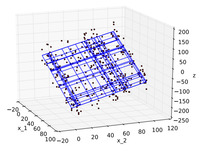
Linear regression ($n=2$)