Logistic regression is a classification method for analyzing a set of data in which there are one or more independent variables (inputs) that determine a binary outcome $0$ or $1$.
Hypothesis function
Suppose that we are given $M$ data samples, denoting the $m$-th observation pair of an input vector and an output by $\mathbf{x}_{m} = \begin{bmatrix} x_0 & x_1 & \cdots & x_n \end{bmatrix}^{T} \in \mathbb{R}^{n+1}$ and $y_{m} \in {0,1}$, respectively. We call $\mathbf{x}_{m}$ a positive sample if $y_{m}=1$ and a negative sample if $y_{m}=0$.
Now, consider $P(y_{m} \vert \mathbf{x}_{m})$, a conditional probability of $y_{m}$ given $\mathbf{x}_{m}$. The hypothesis function $h_{\mathbf{w}}(\mathbf{x}_{m})$ of logistic regression models the conditional probability of a positive sample (i.e., $y_{m}=1$) as
$$ P(y_{m}=1 \vert \mathbf{x}_{m})=h_{\mathbf{w}}(\mathbf{x}_{m}). $$
Here, the hypothesis function $h_{\mathbf{w}}(\mathbf{x}_{m})$ is defined using the sigmoid function $s(z)=\frac{1}{1 + e^{-z}}$ as follows:
$$ h_{\mathbf{w}}(\mathbf{x}_{m})=s(\mathbf{w}^T \mathbf{x}_{m})=\frac{1}{1 + e^{-\mathbf{w}^T \mathbf{x}_{m}}}. $$
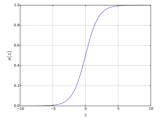
As shown in Figure 1, the sigmoid function $s(z)$ is a ‘S’-shape curve that converges to 1 as $z \rightarrow \infty$ and 0 as $z \rightarrow -\infty$. Since $h_{\mathbf{w}}(\mathbf{x}_{m})$ attempts to model a probability, the property of the sigmoid function $s(z)$ that is bounded between 0 and 1 is a good fit for our purpose.
sigmoid function $s(z)=\frac{1}{1 + e^{-z}}$.
What is next is to choose $\mathbf{w}$ well so that we can have a high value of $h_{\mathbf{w}}(\mathbf{x}_{m})$ for $\mathbf{x}_{m}$ that corresponds to $y_{m}=1$, and a low value for $\mathbf{x}_{m}$ that corresponds to $y_{m}=0$.
Cost function
Since $P(y_{m}=1 \vert \mathbf{x}_{m})=h_{\mathbf{w}}(\mathbf{x}_{m})$ by our definition, we have
$$ P(y_{m}=0 \vert \mathbf{x}_{m})=1-h_{\mathbf{w}}(\mathbf{x}_{m}). $$
For all the observations in the training set, the likelihood $l(\mathbf{w})$ can then be written as
$$ l(\mathbf{w})=\prod_{m=1}^{M} h_{\mathbf{w}}(\mathbf{x}_{m})^{y_{m}} ( 1 - h_{\mathbf{w}}(\mathbf{x}_{m}) )^{1-{y_{m}}}. \tag{logi:1}\label{eq:lr_likelihood} $$
Logistic regression chooses the parameter $\mathbf{w}$ that maximizes the likelihood of observing the samples, represented in \eqref{eq:lr_likelihood}. Thus, we define the cost function $J(\mathbf{w})$ as
$$\scriptsize
\begin{aligned}
J(\mathbf{w})
&= -\frac{1}{M}\log l(\mathbf{w}) \\
&= -\frac{1}{M}\sum_{m=1}^{M} \left( y_{m} \log h_{\mathbf{w}}(\mathbf{x}_{m}) + ( 1-{y_{m}}) \log( 1 - h_{\mathbf{w}}(\mathbf{x}_{m}) ) \right).
\end{aligned}\tag{logi:2}\label{eq:lr_cost}
$$
Note that minimizing \eqref{eq:lr_cost} is equivalent to maximizing \eqref{eq:lr_likelihood}.
Learning
The solution $\mathbf{w}^{*}$ of logistic regression can be obtained by minimizing the cost function in \eqref{eq:lr_cost}. Again, such a minimization can be done by using the gradient descent. Hence, we first obtain the partial derivatives of $J(\mathbf{w})$ as follows:
$$\tiny
\begin{aligned}
&\frac{\partial J(\mathbf{w})}{\partial w_j} \\
&=-\frac{1}{M} \sum_{m=1}^M \left( y_{m} \frac{1}{s(\mathbf{w}^{T} \mathbf{x}_{m})} - (1 - y_{m})\frac{1}{1-s(\mathbf{w}^{T} \mathbf{x}_{m})} \right) \frac{\partial}{\partial w_j}s(\mathbf{w}^{T} \mathbf{x}_{m}) \\
&=-\frac{1}{M} \sum_{m=1}^M \left( y_{m} \frac{1}{s(\mathbf{w}^{T} \mathbf{x}_{m})} - (1 - y_{m})\frac{1}{1-s(\mathbf{w}^{T} \mathbf{x}_{m})} \right) s(\mathbf{w}^{T} \mathbf{x}_{m})(1-s(\mathbf{w}^{T} \mathbf{x}_{m}))\frac{\partial}{\partial w_j}\mathbf{w}^{T} \mathbf{x}_{m}\\
&=-\frac{1}{M} \sum_{m=1}^M \left( y_{m} (1-s(\mathbf{w}^{T} \mathbf{x}_{m})) - (1 - y_{m})s(\mathbf{w}^{T} \mathbf{x}_{m}) \right)x_{m,j} \\
&=\frac{1}{M} \sum_{m=1}^M (h_{\mathbf{w}} (\mathbf{x}_{m})- y_{m})x_{m,j}.
\end{aligned}\label{eq:logistic_derivative}
$$
It is worth noting that the sigmoid function $s(z)$ has an easy-to-calculate derivative: $$\begin{aligned} \frac{ds(z)}{dz}=s(z)(1-s(z)).\end{aligned}$$ Now, the gradient descent equations for logistic regression are
$$
\begin{aligned}
w_{j}^{(t+1)}
&= w_{j}^{(t)}-\frac{\alpha}{M} \sum_{m=1}^{M} (h_{\mathbf{w}^{(t)}} (\mathbf{x}_{m})- y_{m})x_{m,j} \\
&= w_{j}^{(t)}-\frac{\alpha}{M} \sum_{m=1}^{M} \left(\frac{1}{1 + e^{-\mathbf{w}^{(t)T} \mathbf{x}_{m}}}- y_{m} \right)x_{m,j}
\end{aligned}
$$
for all $j$.
Prediction
Given a new input vector $\mathbf{x} = \begin{bmatrix} 1 & x_1 & \ldots & x_n \end{bmatrix}^{T}$, we should predict $y$ in the following rule.
$$
y = \left\{
\begin{matrix}
1 & \text{if } h_{\mathbf{w}^{*}} (\mathbf{x}) \ge 0.5,\\
0 & \text{if } h_{\mathbf{w}^{*}} (\mathbf{x}) < 0.5.\\
\end{matrix} \right.
\tag{logi:3}\label{eq:lr_decision}
$$
That way we can achieve the minimum error rate in classification. (Why? Refer to Bayes decision rule for detailed reason.)
Since $h_{\mathbf{w}^{*}} (\mathbf{x})=s\left(\mathbf{w}^{*T} \mathbf{x}\right)$ and $s(z) \ge 0.5 $ when $z \ge 0$, the decision rule in \eqref{eq:lr_decision} is equivalent to
$$
y = \left\{
\begin{matrix}
1 & \text{if } \mathbf{w}^{*T} \mathbf{x} \ge 0,\\
0 & \text{if } \mathbf{w}^{*T} \mathbf{x} < 0.\\
\end{matrix}
\right.
\label{eq:lr_decision2}
$$
Note that the solution to the linear equation $\mathbf{w}^{*T} \mathbf{x}=0$ is the decision boundary separating the two predicted classes. Figure 2 shows an example where the decision boundary is a line.
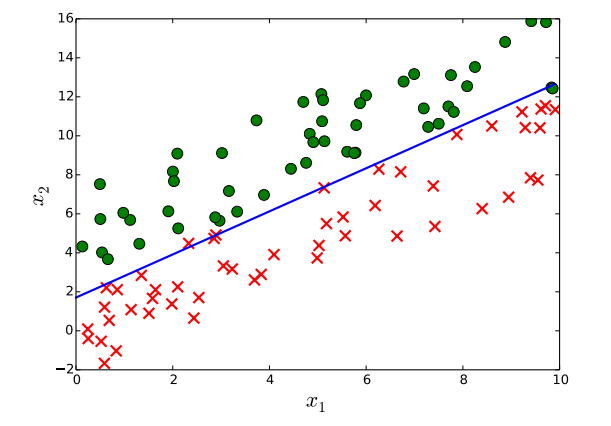
Decision boundary (the blue line) learned by logistic regression separates the data samples, where the green dots and red x’s belong to a different class.
Practice
Figure 2 can be obtained by the following.
import numpy as np
import matplotlib.pyplot as plt
import tensorflow as tf

n_data = 50
r_x = 10
noise_std = 5

class0 = []
class1 = []
x = None
y = None
#--------------------------------------------------------
def create_data():
    global class0, class1, x, y

    slope_1, y_intercept_1 = 1, 5
    slope_2, y_intercept_2 = 1, 0

    for i in range(n_data):
        x_1 = np.random.rand() * r_x
        x_2 = slope_1 * x_1 + y_intercept_1 + (np.random.rand() - 0.5) * noise_std
        class0.append([x_1, x_2, 0])

        x_1 = np.random.rand() * r_x
        x_2 = slope_2 * x_1 + y_intercept_2 + (np.random.rand() - 0.5) * noise_std
        class1.append([x_1, x_2, 1])

    dataset = sorted(class0+class1, key=lambda data: data[0])
    x1, x2, y = zip(*dataset)
    x = np.vstack((np.float32(np.array(x1)), np.float32(np.array(x2))))
    y = np.array(y)
#--------------------------------------------------------
def draw(w, w_0):
    xr = np.arange(0,r_x, 0.1)
    yr  = -(w[0][0] * xr + w_0[0] )/w[0][1]

    for x1, x2, y in class0:
        plt.plot(x1, x2, 'go', markersize=10)

    for x1, x2, y in class1:
        plt.plot(x1, x2, 'rx', markersize=10, mew=2)

    plt.plot(xr, yr, lw=2)
    plt.xlim(0, r_x)
    plt.xlabel('$x_1$', fontsize=20)
    plt.ylabel('$x_2$', fontsize=20)
    plt.gcf().subplots_adjust(bottom=0.15)
    plt.savefig('logistic.pdf')
#--------------------------------------------------------

# Create data
# x of shape [2, n_data], y of shape [1, n_data]
create_data()

# Write a model
w = tf.Variable(tf.random_uniform([1, 2], -1.0, 1.0))
w_0 = tf.Variable(tf.random_uniform([1], -1.0, 1.0))
z = tf.matmul(w, x) + w_0   # w_0 is broadcasted

y_hat = 1 / (1+tf.exp(-z))
cost = -tf.reduce_sum(y*tf.log(y_hat) + (1-y)*(tf.log(1-y_hat))) / len(y)

optimizer = tf.train.GradientDescentOptimizer(0.001)
train = optimizer.minimize(cost)

sess=tf.InteractiveSession()

# Initialize variables
init = tf.initialize_all_variables()
sess.run(init)

# Training
step = 0
while 1:
    try:
        step += 1
        sess.run(train)
        if step % 100 == 0:
            print step, sess.run(cost), sess.run(w), sess.run(w_0)

    # Ctrl+c will stop training
    except KeyboardInterrupt:
        break

# Plot the sample data and decision boundary
draw(sess.run(w), sess.run(w_0))

sess.close()
One versus rest: handling multiclass classification
What if there are more than two classes to classify? What is called the one-versus-rest strategy is a way of extending any binary classifier (including the Logistic regression classifier) to handle multiclass classification problems. The one-versus-rest strategy changes a multiclass classification into multiple binary classifications, training a single classifier per class. The data samples that belongs to a class are treated as positive samples of the class and all others as negative samples.
Consider $y_m={1,2,\ldots,K}$, i.e., we have to decide one out of $K$ classes. Using the Logistic regression as an example, we can make a binary classifier for the class of $y_m=k$ with a corresponding parameter vector $\mathbf{w}_k \in \mathbb{R}^{n+1}$ as
$$ \begin{aligned} \mathbf{h}_{\mathbf{w}_k}(\mathbf{x}_{m}) =\frac{1}{1 + e^{-\mathbf{w}_k^T \mathbf{x}_{m}}} \text{ for } k=1,2,\ldots,K. \end{aligned} $$
The hypothesis function
$\mathbf{h}_{\mathbf{W}}(\mathbf{x}_{m}) \in \mathbb{R}^{K}$ of the
multiclass classification problem can then be expressed as
$$\begin{aligned}
\mathbf{h}_{\mathbf{W}}(\mathbf{x}_{m}) =
\begin{bmatrix}
\mathbf{h}_{\mathbf{w}_1}(\mathbf{x}_{m}) \\
\mathbf{h}_{\mathbf{w}_2}(\mathbf{x}_{m}) \\
\vdots \\
\mathbf{h}_{\mathbf{w}_K}(\mathbf{x}_{m}) \\
\end{bmatrix},\end{aligned}
$$
where $\mathbf{W}$ is a parameter matrix
given as $$\begin{aligned}
\mathbf{W} =
\begin{bmatrix} \mathbf{w}_1 & \mathbf{w}_2 & \cdots & \mathbf{w}_K \end{bmatrix}.\end{aligned}$$
Note that for instance, when $y_m=1$, the first element of
$\mathbf{h}_{\mathbf{W}}(\mathbf{x}_{m})$, namely
$\mathbf{h}_{\mathbf{w}_1}(\mathbf{x}_{m})$, should be high and the
other elements should be low, since samples of the class $y_m=1$ are
treated as positives only for the class $y_m=1$ and as negatives for the
classes $y_m=2,3,\ldots, K$. Roughly speaking, this is achieved by
choosing $\mathbf{W}$ in such a way that
$\mathbf{h}_{\mathbf{W}}(\mathbf{x}_{m})$ is made as close to
$\mathbf{e}_k$ as possible when $y_m=k$, where $\mathbf{e}_k$ is the
$k$-th standard basis vector in $\mathbb{R}^{K}$, that is,
$$\begin{aligned}
\mathbf{e}_1 = \begin{bmatrix} 1 \\
0 \\
\vdots \\
0
\end{bmatrix},
\mathbf{e}_2 = \begin{bmatrix} 0 \\
1 \\
\vdots \\
0
\end{bmatrix},
\ldots,
\mathbf{e}_K = \begin{bmatrix} 0 \\
0 \\
\vdots \\
1
\end{bmatrix}.
\end{aligned}\tag{logi:4}\label{eq:std_basis}$$ Formally, the optimal $\mathbf{W}$
is chosen when we minimize the following cost function:
$$\tiny \begin{aligned} J(\mathbf{W}) = -\frac{1}{M}\sum_{m=1}^{M} \sum_{k=1}^{K} \left( \mathbf{1}_{m}(k) \log h_{\mathbf{w}_k}(\mathbf{x}_{m}) + ( 1-\mathbf{1}_{m}(k)) \log( 1 - h_{\mathbf{w}_k}(\mathbf{x}_{m}) ) \right), \end{aligned}\tag{logi:5}\label{eq:logistic_cost_multi} $$
where $\mathbf{1}_{m}(k)$ is an indicator function, defined as
$$\begin{aligned}
\mathbf{1}_{m}(k) =
\left\{
\begin{matrix}
1 & \text{if } y_{m}=k,\\
0 & \text{if } y_{m} \neq k.
\end{matrix} \right.
\end{aligned}\tag{logi:6}\label{eq:indicator}
$$