Softmax regression is a classification method that generalizes logistic regression to multiclass problems in which possible outcomes are more than two. For this reason, softmax regression is also called multinomial logistic regression.
Generalization from logistic regression
In logistic regression, we have modelled the conditional probabilities as $$\begin{aligned} P(y_{m}=1 \vert \mathbf{x}_{m})=\frac{1}{1 + e^{-\mathbf{w}^T \mathbf{x}_{m}}} \end{aligned} \tag{sm:1}\label{eq:cond1} $$ and $$\begin{aligned} P(y_{m}=0 \vert \mathbf{x}_{m})=\frac{e^{-\mathbf{w}^T \mathbf{x}_{m}}}{1 + e^{-\mathbf{w}^T \mathbf{x}_{m}}}, \end{aligned} \tag{sm:2}\label{eq:cond2} $$ which can be modified to $$\begin{aligned} P(y_{m}=1 \vert \mathbf{x}_{m})=\frac{e^{\mathbf{w}_1^T \mathbf{x}_{m}}}{e^{\mathbf{w}_1^T \mathbf{x}_{m}} + e^{(\mathbf{w}_1-\mathbf{w})^T \mathbf{x}_{m}}} \end{aligned} \tag{sm:3}\label{eq:cond3} $$ and $$\begin{aligned} P(y_{m}=0 \vert \mathbf{x}_{m})=\frac{e^{(\mathbf{w}_1-\mathbf{w})^T \mathbf{x}_{m}}}{e^{\mathbf{w}_1^T \mathbf{x}_{m}} + e^{(\mathbf{w}_1-\mathbf{w})^T \mathbf{x}_{m}}} \end{aligned} \tag{sm:4}\label{eq:cond4} $$
Note that \eqref{eq:cond3} and \eqref{eq:cond4} are made by multiplying $\frac{e^{\mathbf{w}_1^T \mathbf{x}_{m}}}{e^{\mathbf{w}_1^T \mathbf{x}_{m}}}$ to \eqref{eq:cond1} and \eqref{eq:cond2}, respectively. Letting $\mathbf{w}_0=\mathbf{w}_1-\mathbf{w}$, we can rewrite \eqref{eq:cond3} and \eqref{eq:cond4} as follows: $$\begin{aligned} P(y_{m}=k \vert \mathbf{x}_{m})=\frac{e^{\mathbf{w}_k^T \mathbf{x}_{m}}}{\sum_{i=0}^{1} e^{\mathbf{w}_i^T \mathbf{x}_{m}}} \text{ for } k=0,1. \label{eq:cond5}\end{aligned}$$ Thus, the conditional probabilities can be thought of as the ones that exponentiate weighted inputs and then normalize them. In such a sense, softmax regression considers more than two classes, say $K$ of them like $y_{m} \in {1,2,\ldots,K}$, with the model of conditional probabilities in the following: $$\begin{aligned} P(y_{m}=k \vert \mathbf{x}_{m})=\frac{e^{\mathbf{w}_k^T \mathbf{x}_{m}}}{\sum_{i=1}^{K} e^{\mathbf{w}_i^T \mathbf{x}_{m}}} \text{ for } k=1,2,\ldots,K. \label{eq:cond6}\end{aligned}$$ Here, $\mathbf{w}_1, \mathbf{w}_2, \ldots, \mathbf{w}_K \in \mathbb{R}^{n+1}$ are the parameter vectors of our model.
Hypothesis function
Let a parameter matrix $\mathbf{W} \in \mathbb{R}^{(n+1) \times K}$ be
$$ \begin{aligned} \mathbf{W} = \begin{bmatrix} \mathbf{w}_1 & \mathbf{w}_2 & \cdots & \mathbf{w}_K \end{bmatrix}. \end{aligned} $$
Then, we define the hypothesis function of softmax regression, denoted
by $\mathbf{h}_{\mathbf{W}}(\mathbf{x}_{m}) \in \mathbb{R}^{K}$, as
$$\begin{aligned}
\mathbf{h}_{\mathbf{W}}(\mathbf{x}_{m}) =
\begin{bmatrix}
P(y_{m}=1 \vert \mathbf{x}_{m}) \\
P(y_{m}=2 \vert \mathbf{x}_{m}) \\
\vdots \\
P(y_{m}=K \vert \mathbf{x}_{m}) \\
\end{bmatrix}
= \frac{1}{\sum_{i=1}^{K} e^{\mathbf{w}_i^T \mathbf{x}_{m}}}
\begin{bmatrix}
e^{\mathbf{w}_1^T \mathbf{x}_{m}} \\
e^{\mathbf{w}_2^T \mathbf{x}_{m}} \\
\vdots \\
e^{\mathbf{w}_k^T \mathbf{x}_{m}} \\
\end{bmatrix}.\end{aligned}$$ The parameter matrix $\mathbf{W}$ should
be chosen in such a way that for $y_{m}=k$, the $k$-th element of
$\mathbf{h}_{\mathbf{W}}(\mathbf{x}_{m})$ becomes the largest among all
the elements.
Note that $\mathbf{h}_{\mathbf{W}}(\mathbf{x}_{m})$ can be represented
as $$\begin{aligned}
\mathbf{h}_{\mathbf{W}}(\mathbf{x}_{m}) =
\sigma(\mathbf{W}^{T} \mathbf{x}_{m}),\end{aligned}$$ where
$\sigma(\mathbf{z})$ for
$\mathbf{z} = \begin{bmatrix} z_1 & z_2 & \ldots & z_K \end{bmatrix}^{T} \in \mathbb{R}^{K}$
is called the softmax function and is given as $$\begin{aligned}
\sigma(\mathbf{z})=
\begin{bmatrix}
\sigma(\mathbf{z};1) \\
\sigma(\mathbf{z};2) \\
\vdots \\
\sigma(\mathbf{z};K) \\
\end{bmatrix}\end{aligned}$$ with $$\begin{aligned}
\sigma(\mathbf{z};i) = \frac{e^{z_i}}{\sum_{k=1}^{K} e^{z_k}}.
\end{aligned}\tag{sm:5}\label{eq:sm_sigma}$$ The derivatives of the softmax
function have a nice property to remember:
$$\begin{aligned}
\frac{\partial \sigma(\mathbf{z};i)}{\partial z_j}=
\left\{
\begin{matrix}
\sigma(\mathbf{z};i) (1 - \sigma(\mathbf{z};i)) & \text{if } i=j,\\
-\sigma(\mathbf{z};i)\sigma(\mathbf{z};j) & \text{if } i \neq j.\\
\end{matrix} \right.\end{aligned}
$$
Cost function
The likelihood $l(\mathbf{W})$ of all data samples in the training set can be represented as follows: $$\begin{aligned} l(\mathbf{W})=\prod_{m=1}^{M}\prod_{k=1}^{K} \left( \frac{e^{\mathbf{w}_k^T \mathbf{x}_{m}}}{\sum_{i=1}^{K} e^{\mathbf{w}_i^T \mathbf{x}_{m}}} \right)^{\mathbf{1}_{m}(k)}, \label{eq:sm_likelihood}\end{aligned}$$ where the indicator function $\mathbf{1}_{m}(k)$ is the same as (logi:6). Softmax regression attempts to find the parameter matrix $\mathbf{W}$ that maximizes the likelihood $l(\mathbf{W})$. This causes the $k$-th element of $\mathbf{h}_{\mathbf{W}}(\mathbf{x}_{m})$ to be larger than any other when $y_{m}=k$. Towards this end, the cost function is defined in a form of a negative log-likelihood, as in logistic regression:
$$
\begin{aligned}
J(\mathbf{W})
&= -\frac{1}{M}\log l(\mathbf{W}) \\
&= -\frac{1}{M}\sum_{m=1}^{M} \sum_{k=1}^{K}
{\mathbf{1}_{m}(k)} \log\left( \frac{e^{\mathbf{w}_k^T \mathbf{x}_{m}}}{\sum_{i=1}^{K} e^{\mathbf{w}_i^T \mathbf{x}_{m}}} \right).
\end{aligned}\tag{sm:6}\label{eq:sm_cost}
$$
It is worth noting that when $K=2$, \eqref{eq:sm_cost} is equivalent to (logi:5).
Learning
There is no known closed-form solution that minimizes the cost function $J(\mathbf{W})$ in \eqref{eq:sm_cost}. Thus, we can apply the gradient descent here as well. Using the notation in \eqref{eq:sm_sigma}, it is easy to see: $$\small \begin{aligned} \frac{\partial J(\mathbf{W})}{\partial \mathbf{w}_j}= -\frac{1}{M}\sum_{m=1}^{M} \sum_{k=1}^{K} \mathbf{1}_{m}(k) \left(\frac{1}{\sigma(\mathbf{W}^T \mathbf{x}_{m};k)} \cdot \frac{\partial \sigma(\mathbf{W}^T \mathbf{x}_{m};k)}{\partial (\mathbf{w}_j^T \mathbf{x}_{m})} \right) \mathbf{x}_{m} \end{aligned} $$
Focusing on the difference between the term when $k=j$ and the terms when $k \neq j$ of the inner summation, we continue to develop the derivative equation as follows:
$$\tiny
\begin{aligned}
\frac{\partial J(\mathbf{W})}{\partial \mathbf{w}_j}
&=-\frac{1}{M}\sum_{m=1}^{M} \left( \mathbf{1}_{m}(j)(1-\sigma(\mathbf{W}^T \mathbf{x}_{m};j))-\sum_{k \neq j} \mathbf{1}_{m}(k)\sigma(\mathbf{W}^T \mathbf{x}_{m};j) \right) \mathbf{x}_{m} \\
&=-\frac{1}{M}\sum_{m=1}^{M} \left( \mathbf{1}_{m}(j)-\left(\sum_{k=1}^{K} \mathbf{1}_{m}(k) \right)\sigma(\mathbf{W}^T \mathbf{x}_{m};j) \right) \mathbf{x}_{m} \\
&=-\frac{1}{M}\sum_{m=1}^{M} \left( \mathbf{1}_{m}(j)-\sigma(\mathbf{W}^T \mathbf{x}_{m};j) \right) \mathbf{x}_{m}.
\end{aligned}
$$
Therefore, the gradient descent equations of softmax regression are given by $$\begin{aligned} \mathbf{w}_{j}^{(t+1)}=\mathbf{w}_{j}^{(t)}-\frac{\alpha}{M}\sum_{m=1}^{M} \left( \mathbf{1}_{m}(j)-\sigma(\mathbf{W}^{(t)T} \mathbf{x}_{m};j) \right) \mathbf{x}_{m} \end{aligned} $$ for all $j$.
Prediction
Denoting a new input vector by $\mathbf{x} = \begin{bmatrix} 1 & x_1 & \ldots & x_n \end{bmatrix}^{T}$ and the solution by $\mathbf{W}^{*} = \begin{bmatrix} \mathbf{w}_1^{*} & \mathbf{w}_2^{*} & \cdots & \mathbf{w}_K^{*} \end{bmatrix}$, we decide $y=k$ when the largest element of $\mathbf{h}_{\mathbf{W}^{*}}(\mathbf{x})$ is the $k$-th. In other words, the prediction rule is given by: $$\begin{aligned} y=\arg\max_{k}\left( \frac{e^{\mathbf{w}_k^{*T} \mathbf{x}}}{\sum_{i=1}^{K} e^{\mathbf{w}_i^{*T} \mathbf{x}}} \right).\end{aligned}$$
Practice
import numpy as np
import matplotlib.pyplot as plt
import tensorflow as tf
import random
import sys
n_data = 10000
r_x = 10
n_class = 3
n_batch = 10
#---------------------------------------------------------------------
def create_data(n):
"""
This function will make a set of data such that
a random number between c*r_x and (c+1)*r_x is given a label c.
"""
dataset = []
for i in range(n):
c = np.random.randint(n_class)
x_1 = np.random.rand() * r_x + c*r_x
y = c
sample = [x_1, y]
dataset.append(sample)
random.shuffle(dataset)
point_, label_ = zip(*dataset)
_point_ = np.float32(np.array([point_]))
_label_ = np.zeros([n_class, n])
for i in range(len(label_)):
_label_[label_[i]][i] = 1
return _point_, _label_
#---------------------------------------------------------------------
# Create a dataset for training
point, label = create_data(n_data)
# Placeholders to take data in
x = tf.placeholder(tf.float32, [1, None])
y = tf.placeholder(tf.float32, [n_class, None])
# Write a model
w_1 = tf.Variable(tf.random_uniform([n_class, 1], -1.0, 1.0))
w_0 = tf.Variable(tf.random_uniform([n_class, 1], -1.0, 1.0))
y_hat = tf.nn.softmax(w_1 * x + w_0)
cost = -tf.reduce_sum(y*tf.log(y_hat))/n_batch
optimizer = tf.train.GradientDescentOptimizer(0.001)
train = optimizer.minimize(cost)
label_hat_ = tf.argmax(y_hat,0)
correct_cnt = tf.equal(tf.argmax(y,0), label_hat_)
accuracy = tf.reduce_mean(tf.cast(correct_cnt, "float"))
sess = tf.InteractiveSession()
# Initialize variables
init = tf.initialize_all_variables()
sess.run(init)
# Learning
step = 0
while 1:
try:
step += 1
if (n_data == n_batch): # Gradient descent
start = 0
end = n_data
else: # Stochastic gradient descent
start = step * n_batch
end = start + n_batch
if (start >=n_data) or (end >=n_data):
break
batch_xs = point[:, start:end]
batch_ys = label[:, start:end]
train.run(feed_dict={x: batch_xs, y: batch_ys})
if step % 10 == 0:
print step
print w_1.eval()
print w_0.eval()
# With gradient descent, ctrl+c will stop training
except KeyboardInterrupt:
break
# Create another dataset for test
point_t, label_t = create_data(100)
rate = accuracy.eval(feed_dict={x: point_t, y: label_t})
print "\n\n accuracy = %s\n" % (rate)
# Plot the test results
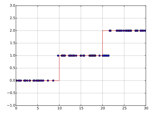
plt.plot(point_t[0,:], label_hat_.eval(feed_dict={x: point_t}), 'o')
plt.grid()
plt.ylim(-1, n_class)
xt = range(0, n_class*10+1, 10)
yt = range(-1, n_class, 1)
plt.step(xt, yt, 'r--')
plt.savefig('softmax_test.pdf')
sess.close()
Figure 1 is what we may get from the code above.