Support vector machine (SVM) is a learning model based on the concept of a separating hyperplane that defines the decision boundary. SVM can be used for both classification and regression analysis, but here we explain it focusing on classification.
Separating hyperplane of the maximum margin
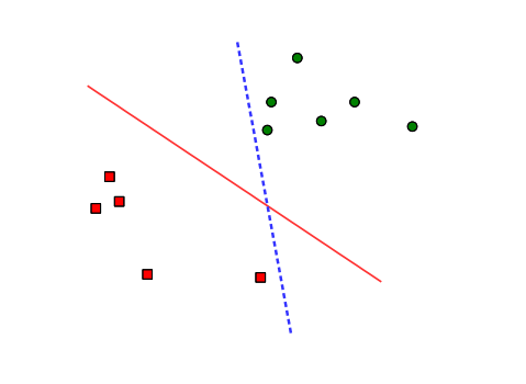
Consider a training set shown in Figure 1, where data samples belong to one of two classes. The separating hyperplane is the decision boundary that divides the two classes by a hyperplane (a line in two dimensions, a plane in three dimensions, and so on). The solid line and the dashed line in the figure are examples of the separating hyperplanes that we can set in this problem. Between the two choices, we may prefer the solid line to the dashed line, because the solid line separates the classes with larger geometric margin and thus it will generalize better to unseen data samples. SVM provides an analytical way to find out the separating hyperplane that has the largest margin. For this reason, a SVM classifier is also called a maximum-margin classifier.
Separating hyperplanes.
Although both the solid and dashed lines can separate the squares from dots, the solid one would be preferred.
Linearly separable classes
Say we are given a training set of $M$ points where the $m$-th input vector is denoted by $\mathbf{x}_{m} \in \mathbb{R}^{n}$ and its corresponding label by $y_{m} \in {-1,1}$. The separating hyperplane can be represented as the set of points $\mathbf{x} \in \mathbb{R}^{n}$ that satisfies the following equation: $$\begin{align} \mathbf{w}^T\mathbf{x}+b=0,\nonumber\end{align}$$ where $\mathbf{w} \in \mathbb{R}^{n}$ and $b \in \mathbb{R}$.1 Note that $\mathbf{w}$ is normal to the hyperplane. If the training samples are linearly separable, we can select two hyperplanes that are parallel to the separating hyperplane and separate the classes without leaving any data samples between them. Without loss of generality, these hyperplanes can be written as
$$ \begin{align} \mathbf{w}^T\mathbf{x}+b=1 \end{align}\tag{svm:1}\label{eq:hyperplane1} $$
and $$ \begin{align} \mathbf{w}^T\mathbf{x}+b=-1. \end{align}\tag{svm:2}\label{eq:hyperplane2} $$
The training samples lying on such hyperplanes are called support vectors. Figure 2 describes the support vectors.
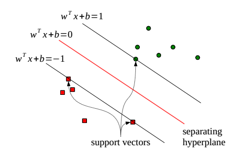
Support vectors.
Now, consider two support vectors $\mathbf{x}_i$ and $\mathbf{x}_j$ such that
$$ \begin{align} \mathbf{w}^T\mathbf{x}_i+b=1 \end{align}\tag{svm:3}\label{eq:sv1} $$
and $$ \begin{align} \mathbf{w}^T\mathbf{x}_j+b=-1, \end{align}\tag{svm:4}\label{eq:sv2} $$
that is, $\mathbf{x}_i$ and $\mathbf{x}_j$ are support vectors that do not belong to the same class. Subtracting \eqref{eq:sv2} from \eqref{eq:sv1} and rescaling with $1/\Vert w \Vert$, we get:
$$ \begin{align} \frac{\mathbf{w}^T}{\Vert w \Vert}(\mathbf{x}_i-\mathbf{x}_j)=\frac{2}{\Vert w \Vert}. \end{align}\tag{svm:5}\label{eq:margin} $$
Note that the projection of a vector $\mathbf{x}_i-\mathbf{x}_j$ onto $\mathbf{w}/\Vert w \Vert$ measures the margin, the distance between the two hyperplanes defined in \eqref{eq:hyperplane1} and \eqref{eq:hyperplane2}. From \eqref{eq:margin}, the margin is equal to $2/\Vert w \Vert$. Therefore, to maximize the margin, we have to minimize $\Vert w \Vert$, which leads to the following optimization problem:
$$
\begin{align}
&\min_{\mathbf{w},b} \frac{\Vert w \Vert^2}{2} \tag{svm:6}\label{eq:svm_opt1} \\
\text{subject to } & y_m (\mathbf{w}^T \mathbf{x}_m+b) \geq 1 \text{ for all } m. \tag{svm:7}\label{eq:svm_opt2}
\end{align}
$$
Learning
Now introducing Lagrange multipliers $\mathbf{\alpha} = \begin{bmatrix} \alpha_1 & \alpha_2 & \cdots & \alpha_M \end{bmatrix}^{T} \in \mathbb{R}^{M}$ for the constraints in \eqref{eq:svm_opt2}, we form the Lagrangian function $L(\mathbf{w},b,\mathbf{\alpha})$ as $$\begin{align} L(\mathbf{w},b,\mathbf{\alpha})=\frac{\Vert w \Vert^2}{2}-\sum_{m=1}^{M} \alpha_m (y_m (\mathbf{w}^T \mathbf{x}_m+b) -1). \tag{svm:8}\label{eq:svm_Lagrangian}\end{align}$$ Then, by Wolfe duality, the solution to \eqref{eq:svm_opt1} can be obtained by solving the following dual problem:
$$
\begin{align}
& \max_{\mathbf{w},b,\mathbf{\alpha}} L(\mathbf{w},b,\mathbf{\alpha}) \tag{svm:9}\label{eq:svm_opt3}\\
\text{subject to } & \frac{\partial}{\partial w_j}L(\mathbf{w},b,\mathbf{\alpha})=0 \text{ for all } m, \tag{svm:10}\label{eq:svm_opt4}\\
& \frac{\partial}{\partial b}L(\mathbf{w},b,\mathbf{\alpha})=0, \tag{svm:11}\label{eq:svm_opt5}\\
& \alpha_m \ge 0 \text{ for all } m \nonumber\label{eq:svm_opt6}
\end{align}
$$
From \eqref{eq:svm_opt4} and \eqref{eq:svm_opt5}, we get $$\begin{align} \mathbf{w}=\sum_{m=1}^{M} \alpha_m y_m \mathbf{x}_m \tag{svm:12}\label{eq:svm_opt7}\end{align}$$ and $$\begin{align} \sum_{m=1}^{M} \alpha_m y_m =0. \tag{svm:13}\label{eq:svm_opt8}\end{align}$$ Substituting \eqref{eq:svm_opt7} and \eqref{eq:svm_opt8} into \eqref{eq:svm_Lagrangian}, we can rewrite the optimization problem in \eqref{eq:svm_opt3} as follows:
$$
\begin{align}
& \max_{\mathbf{\alpha}} \left( \sum_{m=1}^M \alpha_m - \frac{1}{2}\sum_{i=1}^M \sum_{j=1}^M \alpha_i \alpha_j y_i y_j \mathbf{x}_i^T \mathbf{x}_j \right) \tag{svm:14}\label{eq:svm_opt11}\\
& \text{subject to } \sum_{m=1}^{M} \alpha_m y_m =0, \label{eq:svm_opt13} \nonumber \\
& \alpha_m \ge 0 \text{ for all } m \label{eq:svm_opt14} \nonumber
\end{align}
$$
This is a quadratic programming problem with respect to $\mathbf{\alpha}$, and can be solved by a variety of methods (e.g., the conjugate gradient). Having obtained the optimal $\mathbf{\alpha}$, we can determine the optimal $\mathbf{w}$ from \eqref{eq:svm_opt7}.
The optimal $b$ still remains unknown. Now we consider the Karush-Kuhn-Tucker (KKT) complementary slackness conditions, which are given by $$\begin{align} \alpha_m (y_m (\mathbf{w}^T \mathbf{x}_m+b) -1)=0 \text{ for all } m.\nonumber\end{align}$$ From the conditions above, we learn:
$$
\alpha_m = \left\{
\begin{matrix}
0 & \text{if } y_m (\mathbf{w}^T \mathbf{x}_m+b) -1 > 0,\\
\text{non-negative} & \text{if } y_m (\mathbf{w}^T \mathbf{x}_m+b) -1 = 0.\\
\end{matrix} \right.
$$
This means that for non-zero $\alpha_m$ obtained in \eqref{eq:svm_opt11}, the corresponding $\mathbf{x}_m$ are support vectors that satisfy $y_m (\mathbf{w}^T \mathbf{x}_m+b) -1 = 0$. Thus, given a support vector $\mathbf{x}_m$, the optimal value of $b$ can be obtained as $$\begin{align} b=\frac{1}{y_m}-\mathbf{w}^T \mathbf{x}_m. \tag{svm:15}\label{eq:svm_b}\end{align}$$ In practice, we can have a more robust estimate of $b$ by taking an average over various support vectors instead of a single one.
Soft margin: linearly non-separable classes
If the training set is not linearly separable, we will find no feasible solution to \eqref{eq:svm_opt1}. To deal with such a case, we introduce a modification called soft margin. The soft margin method relaxes the constraints in \eqref{eq:svm_opt2} with non-negative slack variables $\xi_m$ as follows:
$$\begin{align} y_m (\mathbf{w}^T \mathbf{x}_m+b) \ge 1- \xi_m \text{ for all } m.\nonumber\end{align}$$
Note that every constraint can be satisfied if $\xi_m$ is sufficiently large. What we actually want is to choose the value of $\xi_m$ to be non-zero only when necessary and as much as necessary. Such a case is when $\mathbf{x}_m$ is an outlier violating the constraint in \eqref{eq:svm_opt2}. The separating hyperplane is then regarded as the solution to the following optimization problem:
$$\small
\begin{align}
&\min_{\mathbf{w},b, \xi_1,\ldots,\xi_M} \left( \frac{\Vert w \Vert^2}{2} +C\sum_{m=1}^M \xi_m \right) \tag{svm:16}\label{eq:svm_soft1} \\
\text{subject to } & y_m (\mathbf{w}^T \mathbf{x}_m+b) \geq 1 -\xi_m \text{ and } \xi_m \ge 0 \text{ for all } m, \tag{svm:17}\label{eq:svm_soft2}
\end{align}$$
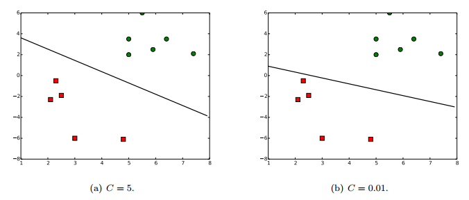
where $C$ is a parameter that controls the solution’s sensitivity to outliers. When $C$ is small, the outliers are almost ignored and large margin is achieved. In contrast, a large $C$ allows a small number of outliers to exist at the cost of narrow margin.
Learning
Define the Lagrangian function $L(\mathbf{w},b,\mathbf{\alpha},\mathbf{\beta})$ as $$\small\begin{align} L(\mathbf{w},b,\mathbf{\alpha},\mathbf{\beta})=\frac{\Vert w \Vert^2}{2}-\sum_{m=1}^{M} \alpha_m (y_m (\mathbf{w}^T \mathbf{x}_m+b) -1+\xi_m)-\sum_{m=1}^{M} \beta_m \xi_m, \label{eq:svm_soft_Lagrangian}\nonumber\end{align}$$ in which $\mathbf{\alpha} = \begin{bmatrix} \alpha_1 & \alpha_2 & \cdots & \alpha_M \end{bmatrix}^{T} \in \mathbb{R}^{M}$ and $\mathbf{\beta} = \begin{bmatrix} \beta_1 & \beta_2 & \cdots & \beta_M \end{bmatrix}^{T} \in \mathbb{R}^{M}$ are Lagrange multipliers. Then, we can have the solution to \eqref{eq:svm_soft1} by solving its Wolfe dual problem given as
$$\begin{align}
& \max_{\mathbf{w},b,\mathbf{\alpha},\mathbf{\beta}} L(\mathbf{w},b,\mathbf{\alpha},\mathbf{\beta}) \tag{svm:18}\label{eq:svm_soft3}\\
\text{subject to } & \frac{\partial}{\partial w_j}L(\mathbf{w},b,\mathbf{\alpha},\mathbf{\beta})=0 \text{ for all } m, \tag{svm:19}\label{eq:svm_soft4}\\
& \frac{\partial}{\partial b}L(\mathbf{w},b,\mathbf{\alpha},\mathbf{\beta})=0, \tag{svm:20}\label{eq:svm_soft5}\\
& \frac{\partial}{\partial \xi_m}L(\mathbf{w},b,\mathbf{\alpha},\mathbf{\beta})=0 \text{ for all } m, \tag{svm:21}\label{eq:svm_soft6}\\
& \alpha_m \ge 0 \text{ and } \beta_m \ge 0 \text{ for all } m. \tag{svm:22}\label{eq:svm_soft7}\end{align}$$
From \eqref{eq:svm_soft6} and \eqref{eq:svm_soft7}, we have
$$\begin{align}
\beta_m = C - \alpha_m \ge 0 \text{ for all } m \nonumber\end{align}$$ and thus
$$\begin{align}
\alpha_m \le C \text{ for all } m.\nonumber\end{align}$$ By substituting
\eqref{eq:svm_soft4}, \eqref{eq:svm_soft5}, and \eqref{eq:svm_soft6} into
\eqref{eq:svm_soft3}, one can show that $\alpha$ is the solution to:
$$\begin{align}
& \max_{\mathbf{\alpha}} \left( \sum_{m=1}^M \alpha_m - \frac{1}{2}\sum_{i=1}^M \sum_{j=1}^M \alpha_i \alpha_j y_i y_j \mathbf{x}_i^T \mathbf{x}_j \right) \nonumber\label{eq:svm_soft11}\\
&\text{subject to } \sum_{m=1}^{M} \alpha_m y_m =0, \nonumber\label{eq:svm_soft12}\\
& 0 \le \alpha_m \le C \text{ for all } m. \nonumber\label{eq:svm_soft13}\end{align}$$
From \eqref{eq:svm_soft4}, the optimal $\mathbf{w}$ is then again
formulated as \eqref{eq:svm_opt7}. To derive the optimal value of $b$, we
can use the KKT complementary slackness conditions as before, which are
given by $$\small\begin{align}
\alpha_m (y_m (\mathbf{w}^T \mathbf{x}_m+b) -1+\xi_m)=0 \text{ and } (C-\alpha_m)\xi_m=0 \text{ for all } m.
\tag{svm:23}\label{eq:svm_kkt}\end{align}$$ Theses conditions imply that if
$0<\alpha_m<C$, we have $\xi_m=0$ and the corresponding $\mathbf{x}_m$
is a support vector. Thus, the optimal $b$ in the soft margin method can
also be estimated as \eqref{eq:svm_b}.
Hinge loss
It is worth noting that we can rewrite \eqref{eq:svm_soft1} and \eqref{eq:svm_soft2} into a form of unconstrained optimization as follows: $$\begin{align} &\min_{\mathbf{w},b} \left( \frac{\Vert w \Vert^2}{2} +C\sum_{m=1}^M \max(0,1-y_m (\mathbf{w}^T \mathbf{x}_m+b)) \right). \tag{svm:24}\label{eq:svm_hinge1}\end{align}$$ In this form, we see that the SVM is also a technique of empirical cost minimization with a regularization term $\Vert w \Vert^2 /2$, where cost function is given by the hinge loss, i.e., $$\begin{align} \text{loss}(y_m, \hat{y}_m) = \max(0, 1-y_m \hat{y}_m)\nonumber\end{align}$$ with $\hat{y}_m=\mathbf{w}^T \mathbf{x}_m+b$. Since \eqref{eq:svm_hinge1} is an unconstrained optimization problem, we can solve it using the gradient descent instead of quadratic programming solvers.
Practice
import numpy as np
import matplotlib.pyplot as plt
import tensorflow as tf

#--------------------------------------------------------
def draw_svm(point, label, w, b, fname):
    for p, y in zip(point, label):
        if (y == -1):
            plt.plot(p[0], p[1], 'go', markersize=10)
        else:
            plt.plot(p[0], p[1], 'rs', markersize=10)

    x = np.arange(1,8,0.1)
    a = -w[0]/w[1]
    y0 = -b/w[1]
    y = a * x + y0
    plt.plot(x, y, 'k-', lw=2)
    plt.savefig(fname)
#--------------------------------------------------------
C = 5.0
_point = [(6.4, 3.5), (7.4, 2.1), (5.0, 3.5), (5.5, 6), (5.9, 2.5),\
         (5, 2), (2.5, -1.9), (4.8, -6.1), (3, -6), (2.3, -0.5), (2.1, -2.3)]
_label = (-1, -1, -1, -1, -1, -1, 1, 1, 1, 1, 1)

x = np.float32(np.array(_point))
y = np.float32(np.transpose(np.array(_label, ndmin=2)))

# Write a model
w = tf.Variable(tf.random_uniform([2, 1], -1.0, 1.0))
b = tf.Variable(tf.random_uniform([1], -1.0, 1.0))
y_hat = tf.matmul(x, w) + b


cost = tf.matmul(tf.transpose(w), w)/2 \
        + C * tf.maximum(tf.constant(0.), tf.constant(1.) - y*y_hat)
optimizer = tf.train.GradientDescentOptimizer(0.001)
train = optimizer.minimize(cost)

sess = tf.InteractiveSession()

# Initialize variables
init = tf.initialize_all_variables()
sess.run(init)

# Learning
step = 0
while 1:
    try:
        step += 1
        sess.run(train)

        if step % 100 == 0:
            print step
            print w.eval()
            print b.eval()

    # Ctrl+c will stop training
    except KeyboardInterrupt:
        break


# Plot the results
draw_svm(_point, _label, w.eval(), b.eval(), 'svm_hinge.pdf')

sess.close()
Figure 3 shows the result of the code above.
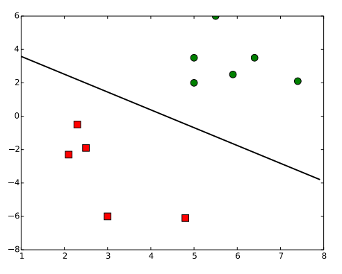
Result of the code above.
Kernel: non-linear SVM
So far we have tried to find a hyperplane that divides data into two classes. However, in practice, we are often confronted with the case where it is by no means reasonable to assume that training set is linearly separable. Figure 4 illustrates such an example. In this case, it is clear that a hyperplane is not a good option to separate classes. Rather, a circle-shape decision boundary would be a better choice.
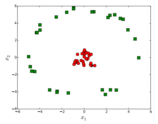
No hyperplane separates data in two dimensions.
A trick to handle this situation is to map data into a higher dimensional space, which we call a feature space. Suppose that we convert the training data using a non-linear mapping $\Phi(\cdot)$ that performs transformation like $$\begin{align} \Phi(\mathbf{x}) \in \mathbb{R}^{n’} \text{ for } \mathbf{x} \in \mathbb{R}^{n},\nonumber\end{align}$$ where $n’>n$. Figure 5 shows an example where a mapping function $\Phi(\mathbf{x})=\begin{bmatrix} x_1 & x_2 & x_1^2+x_2^2 \end{bmatrix}^T$ transforms data in Figure 4 into a feature space of three dimensions.
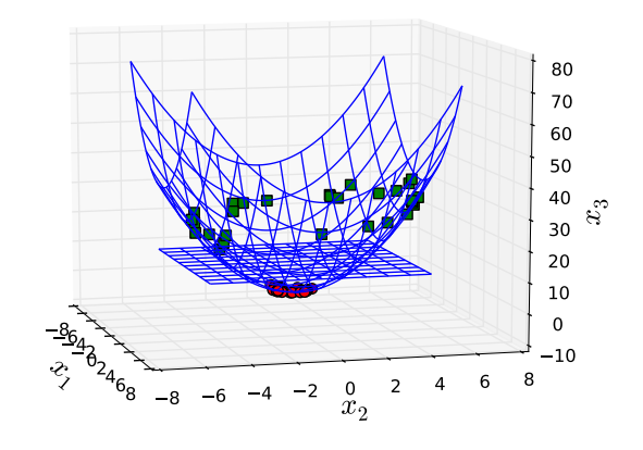
Mapped into three dimensions where there is a hyperplane that separates data.
The data samples in Figure 5 are linearly separable and thus we can find a separating hyperplane instead of a non-linear decision boundary. In general, mapping into a higher-dimension space gives us a possibility to find a linear decision boundary for the case that cannot do otherwise. To apply this trick to SVMs, all we need to do is to replace $\mathbf{x}$ with $\Phi(\mathbf{x})$ in learning equations, e.g., \eqref{eq:svm_opt7}, \eqref{eq:svm_opt11}, and \eqref{eq:svm_b}.
Computation in the feature space is typically costly because it is high dimensional. However, SVMs can avoid this issue by adopting another trick, called kernel trick. Changing $\mathbf{x}$ with $\Phi(\mathbf{x})$, the optimization objective \eqref{eq:svm_opt11} is rewritten as $$\begin{align} \max_{\mathbf{\alpha}} \left( \sum_{m=1}^M \alpha_m - \frac{1}{2}\sum_{i=1}^M \sum_{j=1}^M \alpha_i \alpha_j y_i y_j \Phi(\mathbf{x}_i)^T \Phi(\mathbf{x}_j) \right). \tag{svm:25}\label{eq:svm_opt11r}\end{align}$$ The separating hyperplane, applying \eqref{eq:svm_opt7} and \eqref{eq:svm_b}, is also rewritten as $$\begin{align} \sum_{i=1}^{M} \alpha_i y_i \Phi(\mathbf{x}_i)^T \Phi(\mathbf{x})+\frac{1}{y_m}-\sum_{i=1}^{M} \alpha_i y_i \Phi(\mathbf{x}_i)^T \Phi(\mathbf{x}_m)=0, \tag{svm:26}\label{eq:svm_shpr}\end{align}$$ where $\mathbf{x}_m$ is a support vector. Note from \eqref{eq:svm_opt11r} and \eqref{eq:svm_shpr} that SVMs only depend on data samples through inner products in a feature space. Thus, if we define a kernel function $k(\mathbf{x}_i, \mathbf{x}_j)$ that satisfies $$\begin{align} k(\mathbf{x}_i, \mathbf{x}_j)=\Phi(\mathbf{x}_i)^T \Phi(\mathbf{x}_j),\nonumber\end{align}$$ and calculate the inner products by $k(\mathbf{x}_i, \mathbf{x}_j)$, then we do not even need the mapping explicitly. This use of a kernel function to avoid explicit mapping into a feature space is known as the kernel trick. A choice of the kernel function is on your taste. Only restriction is that the kernel function must be a proper inner product (refer to Mercer’s condition for more detail). One example of a kernel function is $$\begin{align} k(\mathbf{x}_i, \mathbf{x}_j)= e^{-\frac{||\mathbf{x}_i - \mathbf{x}_j||^2}{2\sigma^2}}, \nonumber\end{align}$$ where $\sigma>0$ is a parameter. This is called the (Gaussian) radial basis function kernel, or RBF kernel.
Sequential minimal optimization (SMO)
In the most general version of SVMs, training is solving the quadratic programming (QP) problem described as follows:
$$\begin{align}
& \max_{\mathbf{\alpha}} \Psi(\mathbf{\alpha}) \nonumber\label{eq:smo_soft11}\\
\text{subject to } & \sum_{m=1}^{M} \alpha_m y_m =0, \tag{svm:27}\label{eq:smo_soft12}\\
& 0 \le \alpha_m \le C \text{ for all } m, \nonumber\label{eq:smo_soft13}\end{align}$$
where $$\begin{align}
\Psi(\mathbf{\alpha}) = \sum_{m=1}^M \alpha_m - \frac{1}{2}\sum_{i=1}^M \sum_{j=1}^M \alpha_i \alpha_j y_i y_j k(\mathbf{x}_i, \mathbf{x}_j).
\tag{svm:28}\label{eq:smo_Psi}\end{align}$$ The solution of this problem must
satisfy the KKT conditions in \eqref{eq:svm_kkt}, which we now re-express
as $$\begin{array}{rl}
y_m u_m \ge 1 & \text{if } \alpha_m=0,\\
y_m u_m = 1 & \text{if } 0<\alpha_m<C,\\
y_m u_m \le 1 & \text{if } \alpha_m=C,
\end{array}
\label{eq:smo_kkt}$$ or equivalently
$$\begin{matrix}
y_m e_m \ge 0 & \text{if } \alpha_m=0,\\
y_m e_m = 0 & \text{if } 0<\alpha_m<C,\\
y_m e_m \le 0 & \text{if } \alpha_m=C,\\
\end{matrix}
\tag{svm:29}\label{eq:smo_kkt2}$$
where $u_m$ is the output of the SVM for the $m$-th training sample, i.e., $$\begin{align} u_m=\sum_{j=1}^{M} \alpha_j y_j k(\mathbf{x}_j, \mathbf{x}_m) + b, \tag{svm:30}\label{eq:smo_u}\end{align}$$ and $e_m$ is an error for the $m$-th training sample, defined as $$\begin{align} e_m=u_m-y_m. \tag{svm:31}\label{eq:smo_e}\end{align}$$
Standard numerical QP solvers can be used to solve the QP problem above. However, getting the right solution by using such methods is not that easy because of several practical issues. One example of the issues in practice is memory. The quadratic form of \eqref{eq:smo_Psi} involves a matrix that contains $M^2$ elements, which could be too large to be processed within the memory of a single machine. Think about the case when $M=10000$. Assuming an element is 4 bytes in size, we need 400 Mbytes solely for the matrix.
To avoid such an issue of numerical QP solvers, sequential minimal optimization (SMO) has been proposed as an alternative way to solve the QP problem of SVMs. The SMO breaks the QP problem into a series of smallest possible sub-problems. Because of the constraint \eqref{eq:smo_soft12}, we cannot optimize $\Psi(\mathbf{\alpha})$ with respect to a single Lagrange multiplier $\alpha_m$ with all others fixed. Thus, the smallest possible sub-optimization involves two Lagrange multipliers. In a high level, the SMO is simply summarized as follows:
Pick two Lagrange multipliers $\alpha_i$ and $\alpha_j$.
Optimize $\Psi(\mathbf{\alpha})$ with respect to $\alpha_i$ and $\alpha_j$, holding all other Lagrange multipliers fixed.
Repeat steps 1 and 2 until convergence.
As long as at least one of the two Lagrange multipliers is selected to be the one that violates the KKT conditions, the value of $\Psi(\mathbf{\alpha})$ gets larger (i.e., improved) at each iteration, and thus convergence is guaranteed. (Refer to Osuna’s theorem for more detail.)
Optimization with respect to two Lagrange multipliers
Assume that we are optimizing $\alpha_i$ and $\alpha_j$, while other
Lagrange multipliers are fixed. Because of \eqref{eq:smo_soft12}, we have
$$\begin{align}
y_i \alpha_i+y_j \alpha_j=y_i \alpha_i^{o}+y_j\alpha_j^{o}=-\sum_{m \neq i,j} \alpha_m^{o} y_m.
\tag{svm:32}\label{eq:smo_const}\end{align}$$ Here, the superscript $o$ on a value
means that the value is the old one that was obtained in the previous
iteration. We use this notation throughout the rest of a section.
Because of the relationship of $\alpha_i$ and $\alpha_j$, the feasible
range of $\alpha_j$ is defined as $$\begin{align}
L \le \alpha_j \le H \nonumber\end{align}$$ where $$L = \left\{
\begin{array}{rl}
\max(0,\alpha_j-\alpha_i) & \text{if } y_i \ne y_j\\
\max(C,\alpha_j+\alpha_i-C) & \text{if } y_i = y_j,
\end{array} \right.
\label{eq:bound_L}$$ and $$H = \left\{
\begin{array}{rl}
\min(0,\alpha_j-\alpha_i+C) & \text{if } y_i \ne y_j\\
\min(C,\alpha_j+\alpha_i) & \text{if } y_i = y_j.
\end{array} \right.
\label{eq:bound_H}$$
Multiplying \eqref{eq:smo_const} by $y_i$, we have $$\begin{align} \alpha_i+y_i y_j \alpha_j=\alpha_i^{o}+y_i y_j\alpha_j^{o}=-y_i\sum_{m \neq i,j} \alpha_m^{o} y_m. \nonumber\label{eq:smo_const2}\end{align}$$ Let $s=y_i y_j$ and $$\begin{align} \gamma = \alpha_i^{o}+s \alpha_j^{o}= -y_i\sum_{m \neq i,j} \alpha_m^{o} y_m. \tag{svm:33}\label{eq:smo_const3}\end{align}$$ Then, we can write $\alpha_i$ as $$\begin{align} \alpha_i=\gamma-s \alpha_j. \tag{svm:34}\label{eq:smo_const4}\end{align}$$ Replacing $\alpha_i$ in \eqref{eq:smo_Psi} with $\gamma-s\alpha_j$, we can express the objective function $\Psi(\mathbf{\alpha})$ in terms of $\alpha_j$ as $$\begin{align} \Psi(\mathbf{\alpha}) = \frac{1}{2}\eta \alpha_j^2 + (y_j(e_i^{o}-e_j^{o})- \eta \alpha_j^{o})\alpha_j + \text{constant} \nonumber\end{align}$$ where $$\begin{align} \eta = 2k(\mathbf{x}_i, \mathbf{x}_j)-k(\mathbf{x}_i, \mathbf{x}_i)-k(\mathbf{x}_j, \mathbf{x}_j).\nonumber\end{align}$$ Note $$\begin{align} \frac{\partial^2 \Psi(\mathbf{\alpha})}{\partial \alpha_j^2}=\eta.\nonumber\end{align}$$
If $\eta <0$, the objective function $\Psi(\mathbf{\alpha})$ is maximized when
$$\begin{align} \frac{\partial \Psi(\mathbf{\alpha})}{\partial \alpha_j}=\eta \alpha_j+y_j(e_i^{o}-e_j^{o})- \eta \alpha_j^{o}=0. \tag{svm:35}\label{eq:opt_alpha2}\end{align} $$
Let $\alpha_j^{n}$ be the value of $\alpha_j$ that satisfies \eqref{eq:opt_alpha2}, that is, $$\begin{align} \alpha_j^{n}= \alpha_j^{o} + \frac{y_j(e_j^{o}-e_i^{o})}{\eta}. \tag{svm:36}\label{eq:smo_alpha_2_update}\end{align}$$ If $\alpha_j^{n}$ is not in the feasible range, the maximum is achieved at the boundary that is close to $\alpha_j^{n}$, because $\Psi(\mathbf{\alpha})$ is a quadratic in terms of $\alpha_j$. To sum up, the optimal value of $\alpha_j$, denoted by $\alpha_j^{*}$ is:
$$\alpha_j^{*} = \left\{
\begin{array}{rl}
H & \text{if } \alpha_j^{n} > H\\
\alpha_j^{n} & \text{if } L \le \alpha_j^{n} \le H\\
L & \text{if } \alpha_j^{n} < L.
\end{array} \right.
\label{eq:opt_alpha2_final}
$$
If $\eta=0$, the objective function $\Psi(\mathbf{\alpha})$ is reduced to $$\begin{align} \Psi(\mathbf{\alpha}) = y_j(e_i^{o}-e_j^{o})\alpha_j + \text{constant}.\nonumber\end{align}$$ Since $\Psi(\mathbf{\alpha})$ is a line function in terms of $\alpha_j$, we can achieve its maximum at one of the boundaries of the feasible range: $L$ or $H$. In other words,
$$
\alpha_{j}^{*} =
\left\{
\begin{matrix}
H & \text{if } y_{j}(e_{i}^{o}-e_{j}^{o})L < y_{j}(e_{i}^{o}-e_{j}^{o}) H \\
L & \text{if } y_{j}(e_i^{o}-e_{j}^{o})L > y_{j}(e_{i}^{o}-e_{j}^{o}) H.\\
\end{matrix} \right.
\label{eq:opt_alpha2_final2}
$$
Occasionally, $\Psi(\mathbf{\alpha})$ could be the same at the both ends of the feasible range, which means that we cannot make a progress through this optimization. In such a case, we just set $\alpha_j^{*}=\alpha_j^{o}$.
If $\eta>0$, the objective function $\Psi(\mathbf{\alpha})$ is convex downward and thus there exists no solution. This case may occur with the kernel that does not satisfy Mercer’s conditions.
Meanwhile, from \eqref{eq:smo_const3} and \eqref{eq:smo_const4}, the value of $\alpha_i^{*}$, i.e., the optimal value of $\alpha_i$, can be obtained as: $$\begin{align} \alpha_i^{*} = \alpha_i^{o} +s(\alpha_j^{o}-\alpha_j^{*}).\nonumber\end{align}$$
Update after optimization
Define $\Delta \alpha_i = \alpha_i^{*}-\alpha_i^{o}$ and $\Delta \alpha_j = \alpha_j^{*}-\alpha_j^{o}$. Then, we can update the values of $e_i$, $e_j$, and $b$ in terms of $\Delta\alpha_i$ and $\Delta\alpha_j$.
From \eqref{eq:smo_u} and \eqref{eq:smo_e}, it is easy to see that the new
value of an error $e_m$ is given by $$\begin{align}
e_m=e_m^{o}+\Delta\alpha_i y_i k(\mathbf{x}_i, \mathbf{x}_m) + \Delta\alpha_j y_j k(\mathbf{x}_j, \mathbf{x}_m) + \Delta b.\nonumber\end{align}$$
in which $\Delta b$ is the change in $b$, i.e.,
$\Delta b = b - b^{o}$. In general, from the fact that $e_m=0$ for $m$
such that $0 < \alpha_m < C$, we can obtain $\Delta b$ as
$$\begin{align}
\Delta b=-\left( e_m^{o}+\Delta\alpha_i y_i k(\mathbf{x}_i, \mathbf{x}_m) + \Delta\alpha_j y_j k(\mathbf{x}_j, \mathbf{x}_m) \right).\nonumber\end{align}$$
Thus, in practice, we decide $$\Delta b = \left\{
\begin{array}{rl}
\Delta b_i & \text{if } 0<\alpha_i<C\\
\Delta b_j & \text{if } 0<\alpha_j<C\\
(\Delta b_i+\Delta b_j)/2 & \text{otherwise},
\end{array} \right.
\label{eq:delta_b}$$ where
$\Delta b_m=-\left( e_m^{o}+\Delta\alpha_i y_i k(\mathbf{x}_i, \mathbf{x}_m) + \Delta\alpha_j y_j k(\mathbf{x}_j, \mathbf{x}_m) \right)$.
Note that when both $\alpha_i$ and $\alpha_j$ are at boundaries
(i.e., 0 or $C$), any value between $\Delta b_i$ and $\Delta b_j$
satisfies the KKT conditions and thus we just take the average of
$\Delta b_i$ and $\Delta b_j$.
How to choose two Lagrange multipliers to optimize
In order to accelerate convergence, we use some heuristics to choose two Lagrange multipliers to jointly optimize. The basic idea is to choose $\alpha_j$ in an outer loop that violates KKT conditions and $\alpha_i$ in an inner loop that can result in the largest $\Delta \alpha_j$.
From \eqref{eq:smo_kkt2}, KKT conditions are violated when $$ y_j e_j < 0 \text{ and } \alpha_j<C \label{eq:smo_kkt_violated} $$
or
$$y_j e_j >0 \text{ and } \alpha_j>0. \label{eq:smo_kkt_violated2} $$
When selecting $\alpha_i$, we do not calculate the exact value of $\Delta \alpha_j$. Instead, we estimate it by the absolute value of $e_j^{o}-e_i^{o}$ that comes in \eqref{eq:smo_alpha_2_update}. That way, we can avoid evaluating kernels, which is time-consuming.
There are a few more minor heuristics that were introduced in the original implementation of the SMO algorithm. For details, readers are recommended to refer to Platt’s paper.
Practice
SMO implementation
import random

alpha = []
point = []
label = []
error = []
C = None
M = None
N = None
B = None
tol = 0.001
eps = 0.001
kernel = None
#----------------------------------------------------------
def default_kernel(p1, p2):
    ret = 0
    for q, w in zip(p1, p2):
        ret += q*w
    return ret
#----------------------------------------------------------
def nb_idx_error(i2 = None):
    if i2 == None:
        e2 = 0
    else:
        e2 = error[i2]

    idx_error = [(i, abs(error[i]-e2)) for i in range(len(alpha)) \
                if (alpha[i] > 0) and (alpha[i] < C)]
    return idx_error
#----------------------------------------------------------
def get_weight_linear():
    w = [0]*N
    for m in range(M):
        if (alpha[m] > 0):
            val = alpha[m]*label[m]
            for i in range(N):
                w[i] += val*point[m][i]

    return w
#----------------------------------------------------------
def get_b():
    return B
#----------------------------------------------------------
def get_alpha():
    return alpha
#----------------------------------------------------------
def svm(x):
    svm_out = 0
    for m in range(M):
        svm_out += label[m]*alpha[m]*kernel(point[m], x)
    svm_out += B

    return svm_out
#----------------------------------------------------------
def update_error(i1):
    global error

    error[i1] = svm(point[i1]) - label[i1]

    return error[i1]
#----------------------------------------------------------
def take_step(i1, i2):
    global B, error, alpha

    if (i1 == i2):
        return 0
    alph1 = alpha[i1]
    alph2 = alpha[i2]
    y1 = label[i1]
    y2 = label[i2]
    e1 = update_error(i1)
    e2 = error[i2]
    s = y1*y2

    L = 0
    H = 0
    if (y1 == y2):
        L = max(0, alph2 + alph1 - C)
        H = min(C, alph2 + alph1)
    else:
        L = max(0, alph2 - alph1)
        H = min(C, alph2 - alph1 + C)
    if (L == H):
        return 0

    k11 = kernel(point[i1], point[i1])
    k12 = kernel(point[i1], point[i2])
    k22 = kernel(point[i2], point[i2])
    eta = 2*k12 - k11 - k22
    if (eta < 0):
        a2 = alph2 + y2*(e2-e1)/float(eta)
        if (a2 < L):
            a2 = L
        elif (a2 > H):
            a2 = H
    elif (eta == 0):
        v = y2*(e1-e2)
        obj_L = v*L
        obj_H = v*H

        if (obj_L > obj_H-eps):
            a2 = L
        elif (obj_L < obj_H+eps):
            a2 = H
        else:
            a2 = alph2
    else:
        raise Exception('eta > 0: invalid kernel')

    if abs(a2-alph2) < eps*(a2+alph2+eps):
        return 0

    a1 = alph1 + s*(alph2-a2)

    delta1 = a1 - alph1
    delta2 = a2 - alph2

    # update b
    delta_b = 0
    delta_b1 = -( e1 + delta1*y1*kernel(point[i1],point[i1]) \
                + delta2*y2*kernel(point[i2],point[i1]) )
    delta_b2 = -( e2 + delta1*y1*kernel(point[i1],point[i2]) \
                + delta2*y2*kernel(point[i2],point[i2]) )
    if (a1>0) and (a1<C):
        delta_b = delta_b1
    elif (a2>0) and (a2<C):
        delta_b = delta_b2
    else:
        delta_b = (delta_b1+delta_b2)/2.0
    B += delta_b

    # update errors
    error[i1] += delta1*y1*kernel(point[i1], point[i1]) \
                + delta2*y2*kernel(point[i2], point[i1]) + delta_b
    error[i2] += delta1*y1*kernel(point[i1], point[i2]) \
                + delta2*y2*kernel(point[i2], point[i2]) + delta_b

    # update alphas
    alpha[i1] = a1
    alpha[i2] = a2

    return 1
#----------------------------------------------------------
def examine_example(i2):
    y2 = label[i2]
    alph2 = alpha[i2]
    e2 = update_error(i2)
    r2 = e2*y2
    # do something when there is a Lagrange multiplier that violates KKT conditions
    if (r2<-tol and alph2<C) or (r2>tol and alph2>0):
        idx = []
        idx_error = nb_idx_error(i2)
        if (len(idx_error) > 1):
            idx, error_dif = zip(*idx_error)
            i1 = idx[error_dif.index(max(error_dif))]
            if take_step(i1, i2):
                return 1
            idx = list(idx)
            random.shuffle(idx)

        for i1 in idx:
            if take_step(i1, i2):
                return 1

        seq = range(M)
        random.shuffle(seq)
        for i1 in seq:
            if take_step(i1, i2):
                return 1

    return 0
#----------------------------------------------------------
def main():
    loop_cnt = 0
    num_changed = 0
    examine_all = 1

    # This while-loop terminates
    # when examine_all was 1 and num_changed becomes 0
    # i.e., when KKT conditions hold
    while (num_changed > 0) or (examine_all):
        num_changed = 0
        if (examine_all):
            for m in range(M):
                num_changed += examine_example(m)
        else:
            idx = []
            idx_error = nb_idx_error()
            if (len(idx_error) > 1):
                idx, error_ = zip(*idx_error)
            for i in idx:
                num_changed += examine_example(i)

        if (examine_all):
            examine_all = 0
        elif (num_changed == 0):
            examine_all = 1

        loop_cnt += 1
        print "loop_cnt = " + str(loop_cnt)
#----------------------------------------------------------
def init(_point, _label, _c, _kernel = None):
    global point, label, C, M, N, B, kernel
    point = _point
    label = _label
    C = _c
    M = len(_label)
    N = len(_point[0])
    B = 0
    for m in range(M):
        alpha.append(0.0)
        error.append(-_label[m])

    if (_kernel == None):
        kernel = default_kernel
    else:
        kernel = _kernel
#----------------------------------------------------------
if __name__ == "__main__":
    _point = [(6.4, 3.5), (7.4, 2.1), (5.0, 3.5), (5.5, 6), (5.9, 2.5), (5, 2), \
             (2.5, -1.9), (2.5, -1.9), (4.8, -6.1), (3, -6), (2.3, -0.5), (2.1, -2.3)]
    _label = (-1, -1, -1, -1, -1, -1, 1, 1, 1, 1, 1, 1)
    init(_point, _label, 0.05)
    main()

    print repr(alpha)
    print repr(get_weight_linear())
    print B
SVM training with SMO
import numpy as np
import matplotlib.pyplot as plt
import smo

point = [(6.4, 3.5), (7.4, 2.1), (5.0, 3.5), (5.5, 6), (5.9, 2.5),\
         (5, 2), (2.5, -1.9), (4.8, -6.1), (3, -6), (2.3, -0.5), (2.1, -2.3)]
label = (-1, -1, -1, -1, -1, -1, 1, 1, 1, 1, 1)
C = 5.0
smo.init(point, label, C)
smo.main()

for p, y in zip(point, label):
    if (y == -1):
        plt.plot(p[0], p[1], 'go', markersize=10)
    else:
        plt.plot(p[0], p[1], 'rs', markersize=10)

w = smo.get_weight_linear()
b = smo.get_b()
x = np.arange(1,8,0.1)
a = -w[0]/w[1]
y0 = -b/w[1]
y = a * x + y0
plt.plot(x, y, 'k-', lw=2)
plt.savefig('svm_boundary.pdf')

import numpy as np
import matplotlib.pyplot as plt
import smo
import math
#---------------------------------------------------------------------
def my_kernel(x1, x2):
    x1 = np.array(x1)
    x2 = np.array(x2)
    r = np.linalg.norm(x1-x2)
    ret = math.exp(-pow(r,2)/(2.0*50))
    return ret
#---------------------------------------------------------------------

point = [(6.4, 3.5), (7.4, 2.1), (5.0, 3.5), (5.5, 6), (5.9, 2.5),\
         (5, 2), (2.5, -1.9), (4.8, -6.1), (3, -6), (2.3, -0.5), (2.1, -2.3)]
label = (-1, -1, -1, -1, -1, -1, 1, 1, 1, 1, 1)
C = 20.0


smo.init(point, label, C, _kernel = my_kernel) # try C = 2.0
smo.main()

print "alpha = " + repr(smo.get_alpha())

for p, y in zip(point, label):
    y = smo.svm(p)
    print "y = " + str(y)
    if (y <= -1):
        plt.plot(p[0], p[1], 'go', markersize=10)
    elif (y >= 1):
        plt.plot(p[0], p[1], 'rs', markersize=10)
    else:
        plt.plot(p[0], p[1], 'bx', markersize=10)
plt.xlim(1, 8)
plt.savefig('svm_classification.pdf')
Figure 6 is the result of the code above.
Classfication by SVM.
Notations here are inconsistent with the ones used in other posts: $\mathbf{x}_{m}$ and $\mathbf{w}$ do not contain their zeroth element, $x_{m,0}$ and $w_0$, respectively. This is intended to be consistent with most of other SVM literature.
^