An artificial neural network (ANN) is a machine learning model inspired by biological neural networks in a human brain. ANNs offer an elegant way to formulate a complex non-linear hypothesis, due to their hierarchical virtue of layering non-linear units. Even though possible, using an ANN for regression is considered overkill in many cases. Thus, our discussion will be focused on the use for classification.
Perceptrons
A neuron, illustrated in Figure 1, is a core component of a human brain that transmits electrical signals from one place to others.
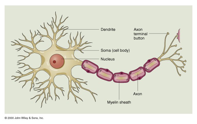
Structure of a biological neuron.
ANN’s neuron, which we call a perceptron, is limited imitation of the real neuron. A perceptron has multiple input channels like dendrites and a single output channel like an axon, as shown in Figure 2.
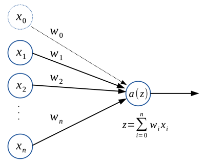
A perceptron.
For given inputs ${ x_{1}, x_{2}, \ldots, x_{n} }$, a perceptron first makes a weighted input $z$, defined as $$\begin{align} z=\sum_{i=0}^{n} w_i x_i,\nonumber\end{align}$$ in which $w_i$ is a weight for an input $x_i$. Here, $x_0$ is called a bias input that is always set to 1, and normally omitted from the illustration of a perceptron. Then, the weighted input $z$ is processed by an activation function $a(z)$ to yield the output. There are many choices to define the activation function. A few examples are listed below:
Sigmoid (or also known as logistic) $$\begin{align} a(z) = \frac{1}{1 + e^{-z}} \tag{ann:1}\label{eq:act_sigmoid}\end{align}$$
Rectified linear unit (often called Relu in short) $$\begin{align} a(z) = \max(0,z)\nonumber\end{align}$$
Hyperbolic tangent $$\begin{align} a(z)=\tanh(z)\nonumber\end{align}$$
As Figure 3 shows, a family of activation functions regulates the output to stay at zero until the weighted input $z$ is larger than a certain threshold at which the output quickly increases.
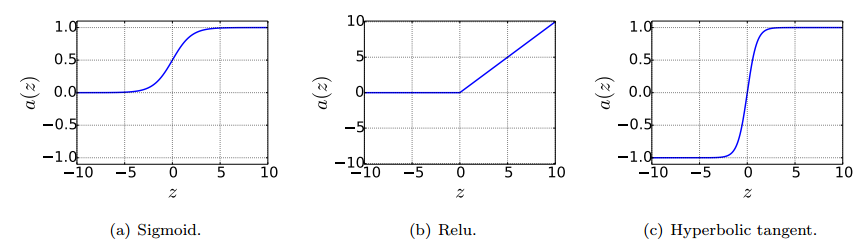
Plots of activation functions.
Structure of ANNs
An ANN is an interconnected group of perceptrons, as exemplified in Figure 4.
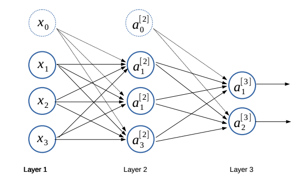
An artificial neural network.
As indicated, outputs of the perceptrons in a layer are fed into the next layer as inputs until the final layer, called an output layer, produces outputs. Here, the first layer is called an input layer where we enter sample observations ${ x_{1}, x_{2}, \ldots, x_{n} }$. The layers between the input layer and output layer are called hidden layers. Adding more hidden layers allows us to model a more complex non-linear function, since the final outputs are composition of multiple activation functions, which are non-linear.
Let $a_i^{[l]}$ be the output of the $i$-th perceptron at layer $l$ with $a_0^{[l]}=1$ (bias units) and $a_i^{[1]}=x_i$ (inputs). Now, we represent the weighted input to the $i$-th perceptron at layer $l$ as $$\begin{align} z_i^{[l]}=\sum_{j=0}^{n^{[l-1]}}w_{ij}^{[l-1]} a_j^{[l-1]},\nonumber\end{align}$$ where $n^{[l-1]}$ is the number of perceptrons at layer $(l-1)$, and $w_{ij}^{[l-1]}$ denotes the weight from the $j$-th perceptron at layer $(l-1)$ to the $i$-th perceptron at layer $l$. Then, we can write $a_i^{[l]}$ as $$\begin{align} a_i^{[l]} = a(z_i^{[l]}).\nonumber\end{align}$$
Multiclass classification
Given an observation pair of an input vector
$\mathbf{x}_{m} = \begin{bmatrix} x_{m,0} & x_{m,1} & \cdots & x_{m,n} \end{bmatrix}^{T} \in \mathbb{R}^{n+1}$
and an output $y_{m} \in {1,2,\ldots,K }$ for $m=1,2,\ldots,M$,
suppose that we want to make a multiclass classifier using an ANN and
the one-versus-rest strategy. Then, since there $K$ classes to classify,
the output layer needs to have $K$ perceptrons, one of which results in
a high value when a corresponding data comes in. The hypothesis function
is simply the vector that represents the output layer. That is, assuming
that there are $L$ layers, the hypothesis function
$\mathbf{h}_{\mathbf{W}}(\mathbf{x}_{m})$ is given as $$\begin{align}
\mathbf{h}_{\mathbf{W}}(\mathbf{x}_{m})=
\begin{bmatrix}
a_{m,1}^{[L]} \\
a_{m,2}^{[L]} \\
\vdots \\
a_{m,K}^{[L]} \\
\end{bmatrix},\nonumber\end{align}$$ where $\mathbf{W}$ is a set of all weights
${ w_{ij}^{[l]} }$, and $a_{m,i}^{[l]}$ denotes $a_{i}^{[l]}$ when
$\mathbf{x}_{m}$ is entered into an ANN. For example, if the activation
functions are defined by the sigmoid in \eqref{eq:act_sigmoid}, what we
need to do for training is to choose $w_{ij}^{[l]}$ for all $i,j,l$ so
that $\mathbf{h}(\mathbf{x}_{m})$ gets close to $\mathbf{e}_k$ given in
(logi:4) when $y_m=k$. Similarly to (logi:5), the cost function $J(\mathbf{W})$ is
then defined as $$\begin{align}
J(\mathbf{W})
= \frac{1}{M}\sum_{m=1}^{M} J_m(\mathbf{W}),
\label{eq:nn_cost_multi}\nonumber\end{align}$$ where $$\begin{align}
J_m(\mathbf{W})
= -\sum_{k=1}^{K}
\left( \mathbf{1}_{m}(k) \log(a_{m,k}^{[L]}) + ( 1-\mathbf{1}_{m}(k)) \log( 1 - a_{m,k}^{[L]} ) \right).
\label{eq:nn_cost_multi2}\nonumber\end{align}$$
Backpropagation
In order to have the optimal $\mathbf{W}$, we need to minimize the cost function $J(\mathbf{W})$, which can be done by using the gradient descent. In this case, the gradient descent equations are
$$ \begin{align} w_{ij}^{[l](t+1)} = w_{ij}^{[l](t)} - \alpha \left. \frac{\partial J(\mathbf{W})}{\partial w_{ij}^{[l]}} \right \vert_{\mathbf{W}=\mathbf{W}^{(t)}} \tag{ann:2}\label{eq:ann_gd}. \end{align} $$
However, it is not easy to derive a closed-form of $\partial J(\mathbf{W}) / \partial w_{ij}^{[l]}$, since $J(\mathbf{W})$ is a composite function of sigmoids. For this reason, training an ANN is conducted in conjunction with backpropagation.
The backpropagation, an abbreviation for “backward propagation of
errors”, provides an alternative way to compute
$\partial J(\mathbf{W}) / \partial w_{ij}^{[l]}$. To see this, we first
define an error $\delta_{m,i}^{[l]}$ of the $i$-th perceptron at layer
$l$ according to $\mathbf{x}_{m}$ as $$\begin{align}
\delta_{m,i}^{[l]} = \frac{\partial J_m(\mathbf{W})}{\partial z_{m,i}^{[l]}},
\tag{ann:3}\label{eq:ann_bp0}\end{align}$$ in which $z_{m,i}^{[l]}$ denotes
$z_{i}^{[l]}$ when $\mathbf{x}_{m}$ comes into the network. Then, we
first note that $$\begin{align}
\frac{\partial J(\mathbf{W})}{\partial w_{ij}^{[l]}}
&= \frac{1}{M}\sum_{m=1}^{M} \frac{\partial J_m(\mathbf{W})}{\partial w_{ij}^{[l]}} \nonumber\\
&= \frac{1}{M}\sum_{m=1}^{M} \frac{\partial z_{m,i}^{[l+1]}}{\partial w_{ij}^{[l]}}\frac{\partial J_m(\mathbf{W})}{\partial z_{m,i}^{[l+1]}} \nonumber\\
&=\frac{1}{M}\sum_{m=1}^{M}a_{m,j}^{[l]} \delta_{m,i}^{[l+1]}. \tag{ann:4}\label{eq:ann_bp1}\end{align}$$
This means that since $a_{m,j}^{[l]}$ is a known value (computed through
the ANN), $\partial J(\mathbf{W}) / \partial w_{ij}^{[l]}$ can be
calculated by obtaining $\delta_{m,i}^{[l+1]}$.
In the meantime, using a chain rule, we have $$\begin{align}
\delta_{m,i}^{[l]} & = \frac{\partial J(\mathbf{W})}{\partial z_{m,i}^{[l]}} \nonumber\\
& = \sum_k \frac{\partial J(\mathbf{W})}{\partial z_{m,k}^{[l+1]}} \frac{\partial z_{m,k}^{[l+1]}}{\partial z_{m,i}^{[l]}} \nonumber\\\
& = \sum_k \delta_{m,k}^{[l+1]} \frac{\partial z_{m,k}^{[l+1]}}{\partial z_{m,i}^{[l]}}.\nonumber\end{align}$$
Since
$z_{m,k}^{[l+1]} = \sum_r w_{kr}^{[l]} a_{m,r}^{[l]} = \sum_r w_{kr}^{[l]} a(z_{m,r}^{[l]})$,
we know $$\begin{align}
\frac{\partial z_{m,k}^{[l+1]}}{\partial z_{m,i}^{[l]}} = w_{ki}^{[l]} a’(z_{m,i}^{[l]}).\nonumber\end{align}$$
Therefore, we can represent $\delta_{m,i}^{[l]}$ as $$\begin{align}
\delta_{m,i}^{[l]} = a’(z_{m,i}^{[l]}) \sum_k \delta_{m,k}^{[l+1]} w_{ki}^{[l]}.
\tag{ann:5}\label{eq:ann_bp2}\end{align}$$ Notice in \eqref{eq:ann_bp2} that
$a’(z_{m,i}^{[l]})$ and $w_{ki}^{[l]}$ are all known. Thus, we see that
$\delta_{m,i}^{[l]}$ is determined by $ \delta_{m,k}^{[l+1]}$ for all
$k$. In other words, once we know $\delta_{m,i}^{[L]}$ for all $i$, then
we can compute $\delta_{m,i}^{[L-1]}$, $\delta_{m,i}^{[L-2]}$, $\ldots$,
$\delta_{m,i}^{[2]}$ for all $i$ iteratively using \eqref{eq:ann_bp2}.
Fortunately, we can easily compute $\delta_{m,i}^{[L]}$, expressing it
in terms of the output activation, $$\begin{align}
\delta_{m,i}^{[L]} &= \frac{\partial J_m(\mathbf{W})}{\partial a_{m,i}^{[L]}} \frac{\partial a_{m,i}^{[L]}}{\partial z_{m,i}^{[L]}} \nonumber\\
&= \frac{\partial J_m(\mathbf{W})}{\partial a_{m,i}^{[L]}} a’(z_{m,i}^{[L]}). \tag{ann:6}\label{eq:ann_bp3}\end{align}$$
Here, $a’(z_{m,i}^{[L]})$ is known, and
$\partial J_m(\mathbf{W})/\partial a_{m,i}^{[L]}$ can also be calculated
without difficult, since $J_m(\mathbf{W})$ is a function of
$a_{m,i}^{[L]}$.
In summary, backpropagation represented by four equations \eqref{eq:ann_bp0}, \eqref{eq:ann_bp1} \eqref{eq:ann_bp2}, and \eqref{eq:ann_bp3}, is an algorithm to compute $\delta_{m,i}^{[l]}$ iteratively from $l=L$ to $l=2$, by which we can eventually obtain $\partial J(\mathbf{W}) / \partial w_{ij}^{[l]}$. Now, the gradient descent with backpropagation can be stated as follows.
Choose the initial value of $w_{ij}^{[l]}$ randomly.
Do the following for $m=1,2,\ldots,M$.
Set $a_{m,i}^{[1]} = x_{m,i}$.
Perform forward propagation to compute $a_{m,i}^{[l]}$ for $l = 2,3,\dots ,L$.
Perform backpropagation to compute $\delta_{m,i}^{[l]}$ for $l = L, L-1,\dots ,2$.
Set $\frac{\partial J(\mathbf{W})}{\partial w_{ij}^{[l]}}=\frac{1}{M}\sum_{m=1}^{M}a_{m,j}^{[l]} \delta_{m,i}^{[l+1]}$.
Update $w_{ij}^{[l]}$ using \eqref{eq:ann_gd}.
Repeat steps 2 to 4 until convergence.
Practice
import numpy as np
import matplotlib.pyplot as plt
import tensorflow as tf
import random
import sys
n_data = 10000
r_x = 10
n_class = 3
#---------------------------------------------------------------------
def create_data(n):
"""
This function will make a set of data such that
a random number between c*r_x and (c+1)*r_x is given a label c.
"""
dataset = []
for i in range(n):
c = np.random.randint(n_class)
x_1 = np.random.rand() * r_x + c*r_x
y = c
sample = [x_1, y]
dataset.append(sample)
random.shuffle(dataset)
point_, label_ = zip(*dataset)
_point_ = np.float32(np.array([point_]))
_label_ = np.zeros([n_class, n])
for i in range(len(label_)):
_label_[label_[i]][i] = 1
return _point_, _label_
#---------------------------------------------------------------------
# Create a dataset for training
point, label = create_data(n_data)
# Placeholders to take data in
x = tf.placeholder(tf.float32, [1, None])
y = tf.placeholder(tf.float32, [n_class, None])
# Write a model
w1 = tf.Variable(tf.random_uniform([4, 1], -1.0, 1.0))
w1_0 = tf.Variable(tf.random_uniform([4, 1], -1.0, 1.0))
layer2 = tf.sigmoid(tf.matmul(w1, x) + w1_0)
w2 = tf.Variable(tf.random_uniform([n_class, 4], -1.0, 1.0))
w2_0 = tf.Variable(tf.random_uniform([n_class, 1], -1.0, 1.0))
layer3 = tf.sigmoid(tf.matmul(w2, layer2) + w2_0)
cost = -tf.reduce_sum(y*tf.log(layer3)+(1-y)*tf.log(1-layer3))/n_data
optimizer = tf.train.GradientDescentOptimizer(0.001)
train = optimizer.minimize(cost)
# Compute accuracy
label_hat_ = tf.argmax(layer3,0)
correct_cnt = tf.equal(tf.argmax(y,0), label_hat_)
accuracy = tf.reduce_mean(tf.cast(correct_cnt, "float"))
sess = tf.InteractiveSession()
# Initialize variables
init = tf.initialize_all_variables()
sess.run(init)
# Learning
step = 0
while 1:
try:
step += 1
train.run(feed_dict={x: point, y: label})
if step % 100 == 0:
print step
print w1.eval()
print w1_0.eval()
print w2.eval()
print w2_0.eval()
# Ctrl+c will stop training
except KeyboardInterrupt:
break
# Create another dataset for test
point_t, label_t = create_data(100)
rate = accuracy.eval(feed_dict={x: point_t, y: label_t})
print "\n\n accuracy = %s\n" % (rate)
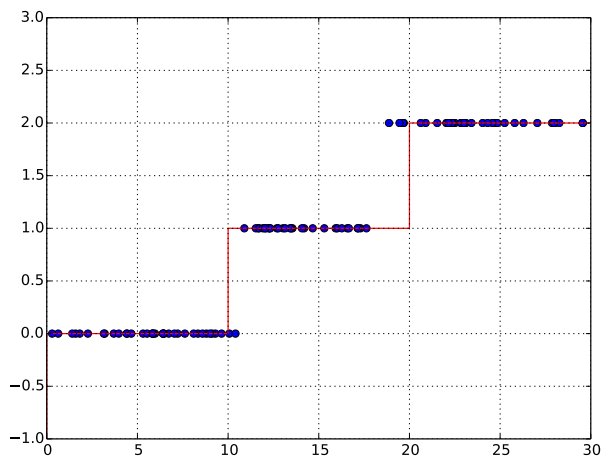
# Plot the test results
plt.plot(point_t[0,:], label_hat_.eval(feed_dict={x: point_t}), 'o')
plt.grid()
plt.ylim(-1, n_class)
xt = range(0, n_class*10+1, 10)
yt = range(-1, n_class, 1)
plt.step(xt, yt, 'r--')
plt.savefig('ann_test.pdf')
sess.close()
Figure 5 is what you may get from the code above.